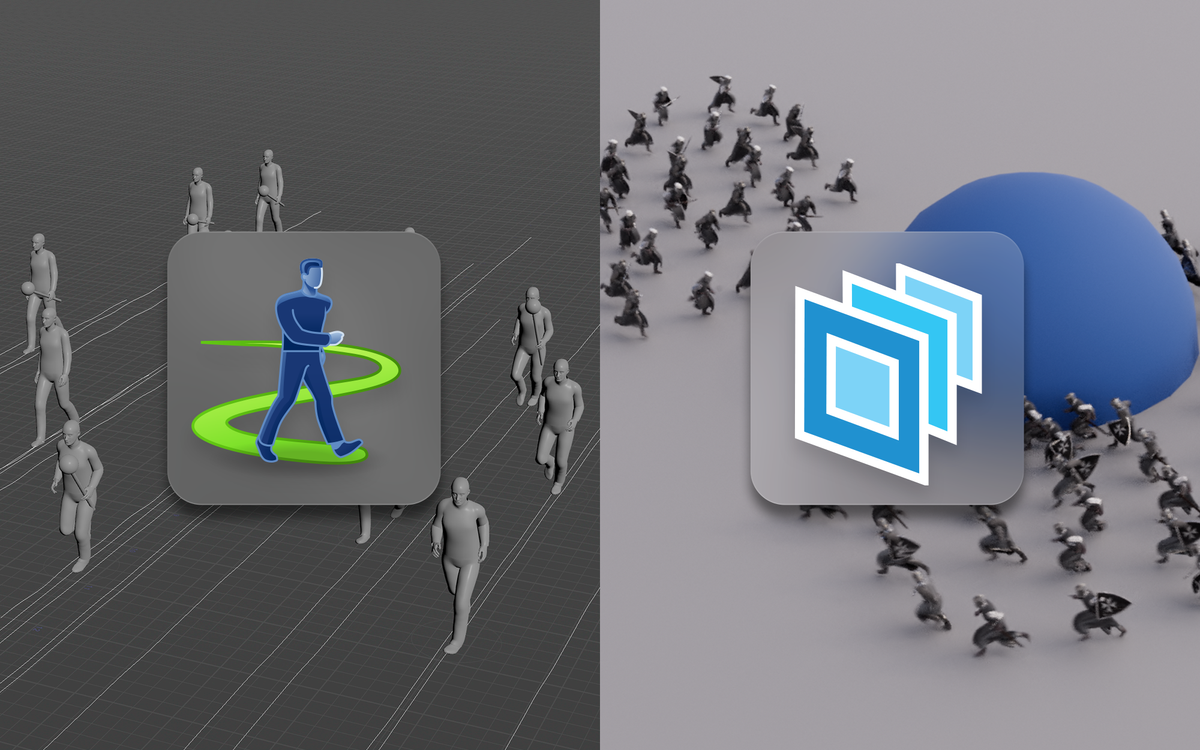
Efficient Vegetation Simulation and Layout using Auto-rigged Agents in Houdini (Part 1/2)
Recently I've been playing around with vegetation in Houdini. One of my main goals was to find a system for efficiently extracting vegetation from an existing layout, and layer animation on top through UsdSkel.
The primary use-case for this is for characters walking through dense vegetation, where you need to extract specific instances of vegetation to simulate collisions.
For this, I designed a system for turning vegetation into agents, automatically creating an approximate skeleton ready for simulation with Vellum. The idea is that you would use these agents directly in the point instancer of the layout, from which you could then hand-pick specific pieces of vegetation for simulation. Since they are agents, you would be able to extract the skeleton, use that as an input for a Vellum simulation, and simply re-attach the animated pose to the agent - outputting very lightweight animated caches utilizing the UsdSkel.
This first part covers the automatic batch generation of vegetation agents with proxies, shaders, and skeletons, ready for simulation with Vellum - and rendering in Houdini with Karma.
Part two will cover setting up our layout, simulation in Vellum, and finally rendering and compositing the final result you see below.
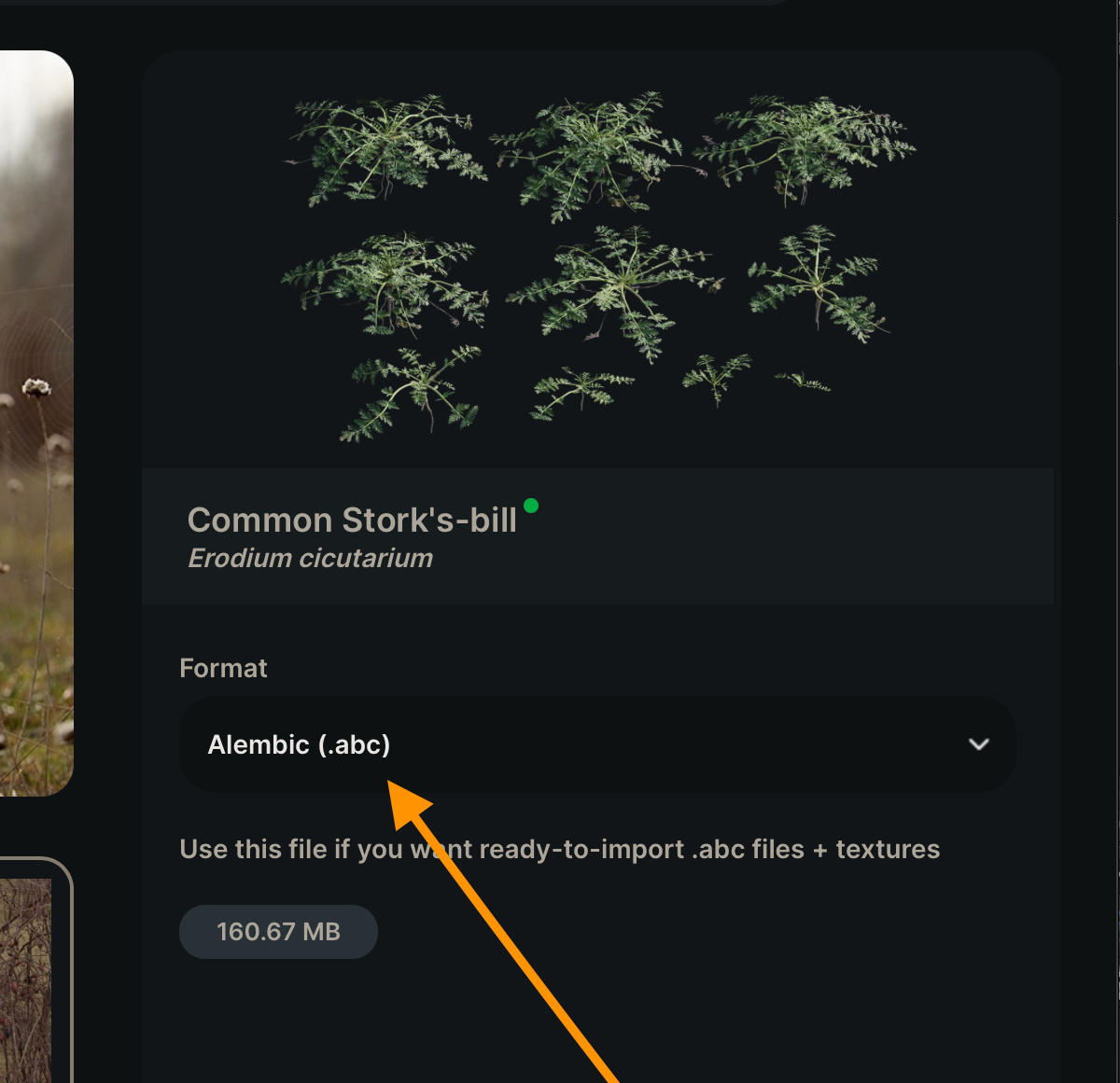
If you want to follow along you can download any of the wonderful free vegetation assets found on gscatter.com . Just make sure to download the Alembic version of the assets. If the vegetation asset contains an alembic called "Building Blocks" I recommend deleting that file before proceeding as you'll otherwise get a very large amount of additional assets (one for each "building block").
The primary vegetation asset I'll be using for this demo is the "Blackberry RubusPlicatus" - you can download it here: https://store.gscatter.com/assets?search=blackberry&workspace=
Final composited shot.
Initial PDG Setup
TOPs network for batch asset generation
Before we start diving into rig generation, I wanted to set up a basic PDG network that runs over each of our downloaded vegetation assets. Setting this up before we begin will allow us to quickly switch between different assets and make sure our agent generation works across different vegetation types. This will be the network we use to export our final USD files as well.
If you're unfamiliar with PDG/TOPs, I highly recommend checking out the Houdini documentation here.
You can either jump to the /tasks context, or create a TOP Network in /obj. I chose the latter in my case.
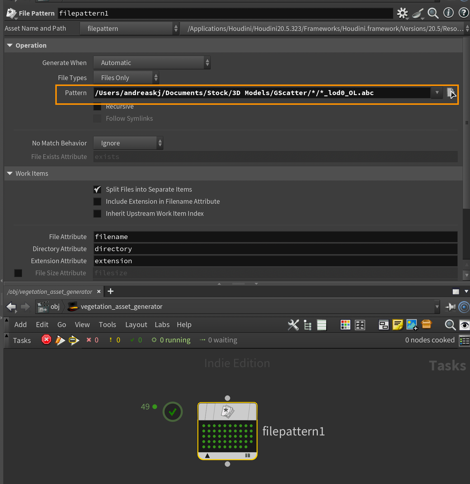
Inside the TOP network, I created a File Pattern node. This node is able to look through a pattern and creates a work item for every file on your system that matches that pattern. It also creates some useful attributes like filename, directory, and extension that we'll use shortly.
I set the pattern to /Users/andreaskj/Documents/Stock/3D Models/GScatter/*/*_lod0_OL.abc in my case. This will target every subfolder of my GScatter folder and subsequently every ld0_0l.abc file, which is what the highest resolution GScatter alembic files are called. If you're using Megascans or something else you'll need to change this pattern accordingly.
If you now select the File Pattern node and press SHIFT+V to Dirty and Cook the node, you should get a work item (represented by the green dots) for each lod0 alembic model in the specified directories. If you middle-click one of the green dots you can check the attributes generated for each work item.
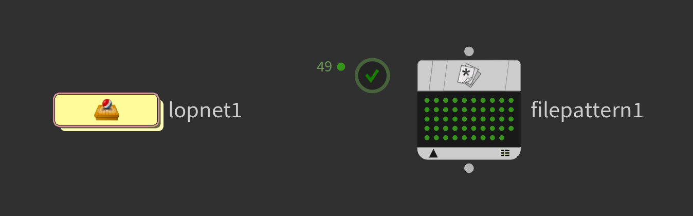
Left-click one of the dots/work items to set that as the current context. Doesn't matter which one. This will allow us to work specifically on that piece of vegetation, and also gives us a nice dropdown to select other work items once we're inside another context.
Still inside the TOPs network, create a LOP network. We will use this to make the asset generation setup that we'll later execute from TOPs.
Inside the LOP network, we need to set up a Component Builder network. This will allow us to do easy processing of USD assets and author everything in a clean way following USD standards. You can simply add the Component Builder recipe from the TAB menu, and you'll get everything you need. For now, we won't do anything else with this, but later, once we need to add shaders and variants, we'll revisit it.
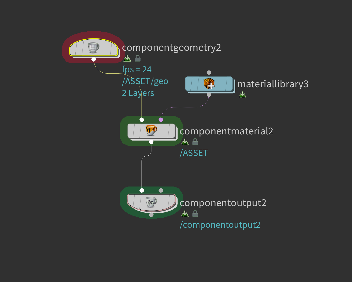
Finally, jump inside the Component Geometry node and we can get started with our Agent Generation in SOPs.
Agent Generation
Auto-rigging and generating agents based on input vegetation models.
One of the main challenges I encountered with animating vegetation was the need to create good skeletons based on our input geometry. This can quickly turn into a very time-consuming task, especially when dealing with the large amount of different vegetation often found in environments.
Some vegetation modelling packages, like Speed Tree, can output some variation of a skeleton that can be used for rigging. But oftentimes in production you'll find yourself using models from providers such as Megascans or GScatter. These rarely have skeletons or curves you can use for deformation, which establishes a need for us to create our own custom skeletons.
In this section I'll present an approach to generating these agent-ready skeletons automatically.
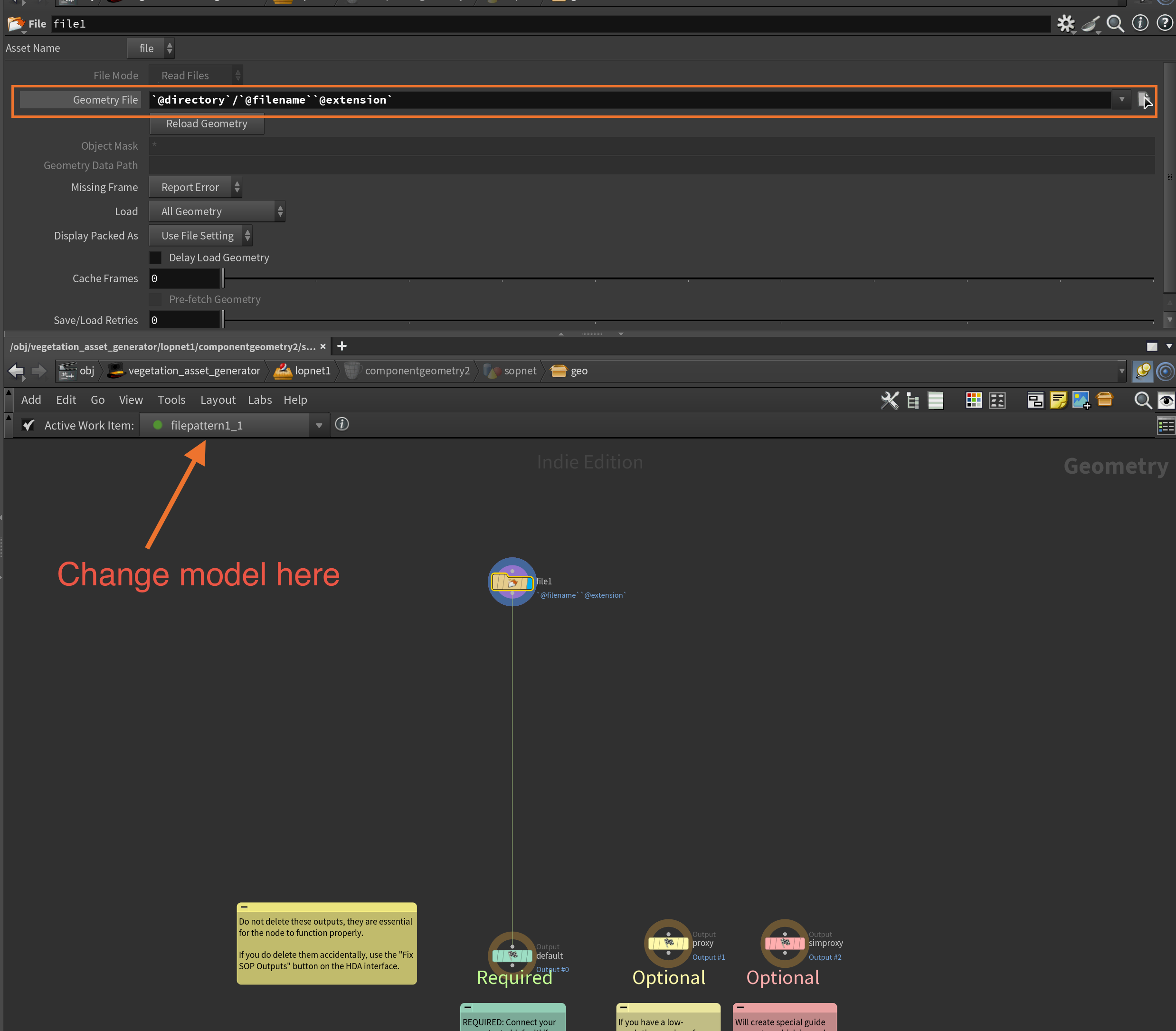
Inside the Component Geometry node drop down a File SOP and connect it to the default output node. This will be our Render geometry.
For the Geometry File, change this to:
`@directory`/`@filename``@extension`These are the attributes generated by our TOPs network. You can use the dropdown seen in the screenshot below to switch to different work items/models. If you don't see the dropdown, make sure you've set an active work item in your TOPs network by left-clicking a work item (the little dots in the cooked TOP node) as described in the previous section.
Next, I created a subnetwork called agent_generate for organisation purposes, and added it underneath the File SOP. Dive into this newly created subnetwork and we can start setting up the agent generator.
Skeleton Generation
In order to turn our vegetation into agents, we need 2 components - a skeleton and a mesh with weights based on said skeleton.
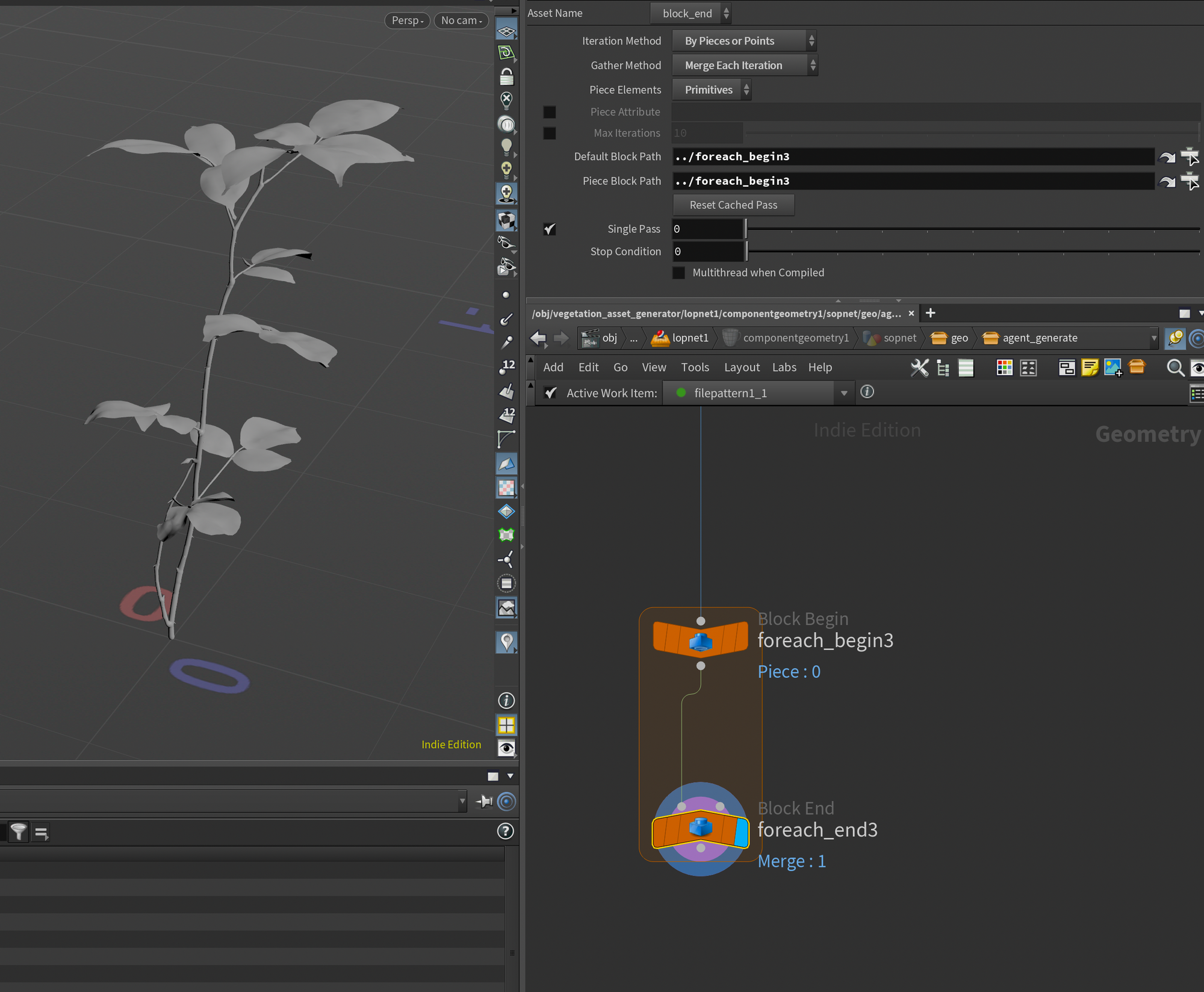
Since our .abc from GScatter contains multiple models, we'll need to create a for each primitive and generate a unique agent for each model. For now, I'll also set the Single Pass to 0 so we can focus on testing our setup on one of the models.
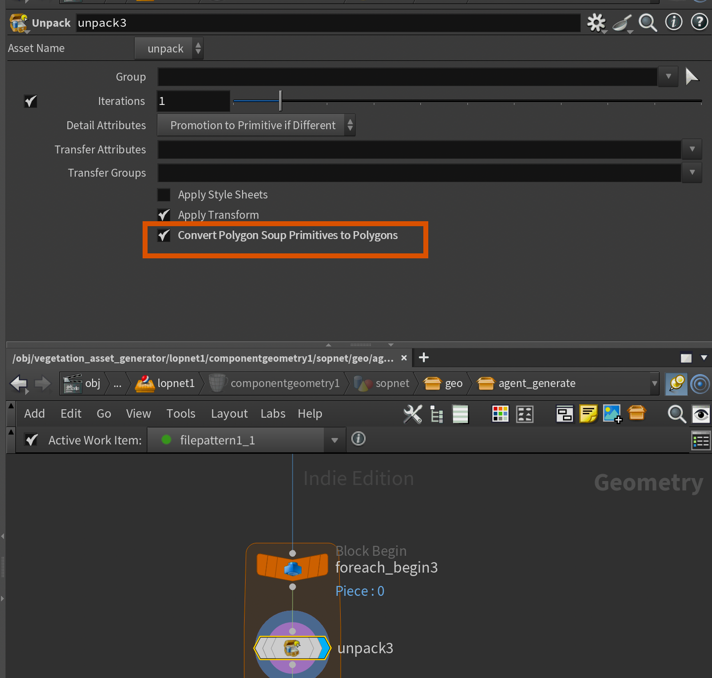
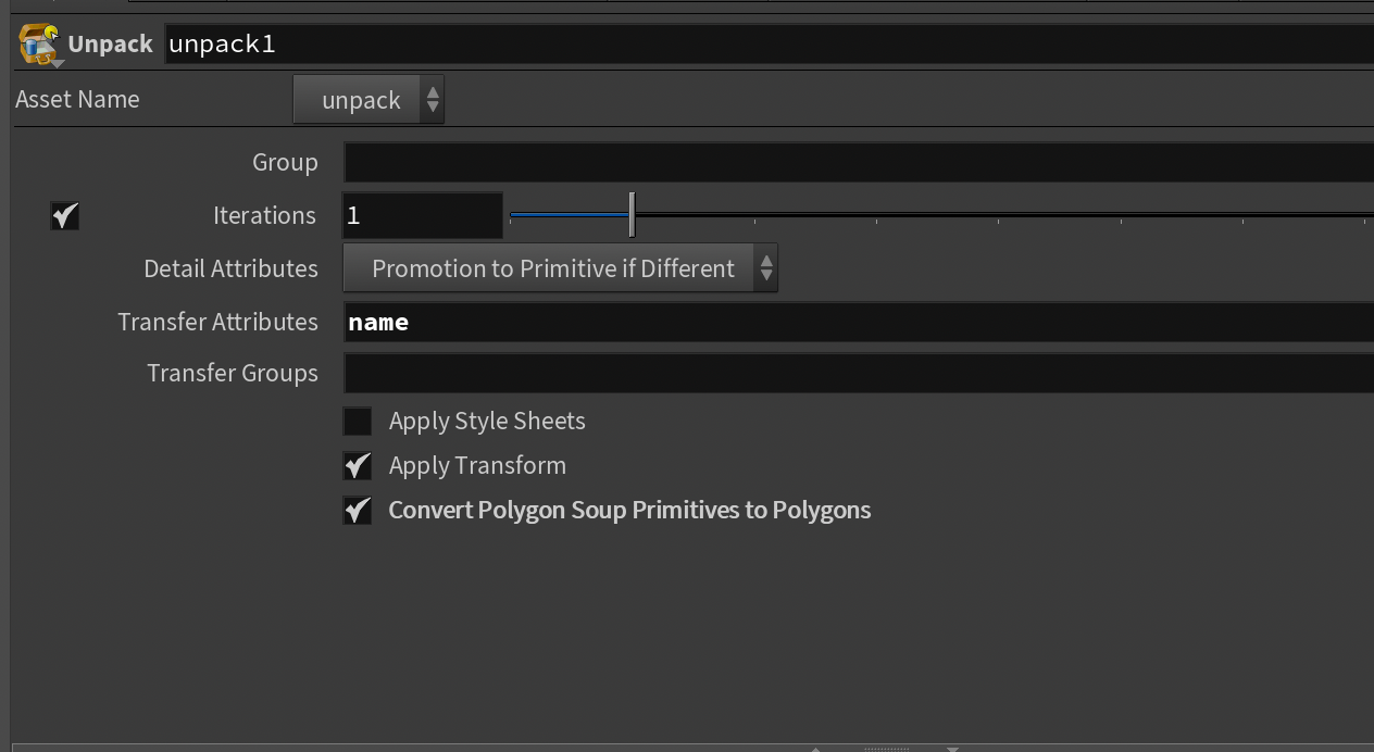
In order for our skeleton generation to work properly we'll need to first unpack the geometry using an Unpack node. Remember to toggle Convert Polygon Soup Primitives to Polygons as we need the raw geometry for generating our skeletons.
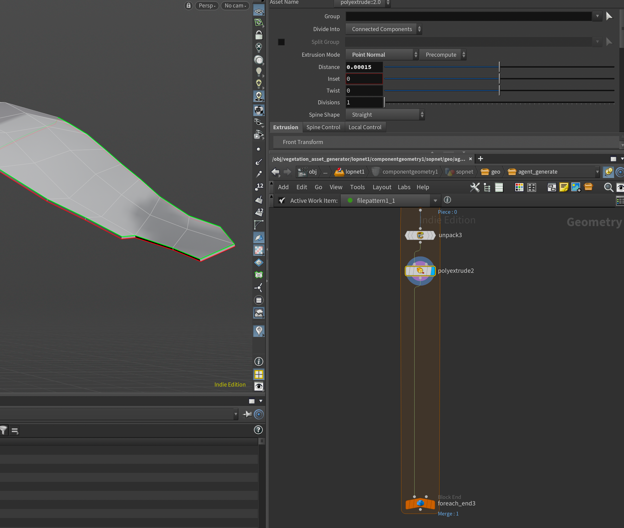
Finally, I extrude all geometries by a tiny amount with a Poly Extrude. This is in order to help the skeleton generator a bit, as it works best with meshes that have a bit of thickness.
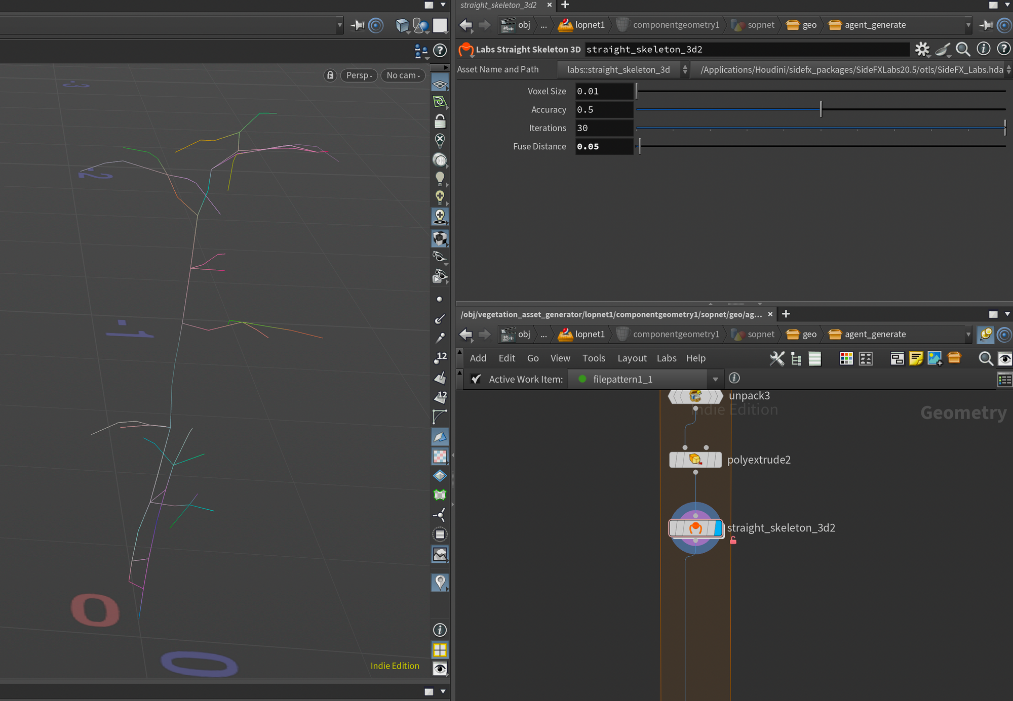
Now it's time to generate our skeletons. I tried several different techniques, even tried to build my own generator. But eventually I ended up settling with the built-in Labs Straight Skeleton 3D . This node works surprisingly well, and just needed a tiny adjustment for my use-case.
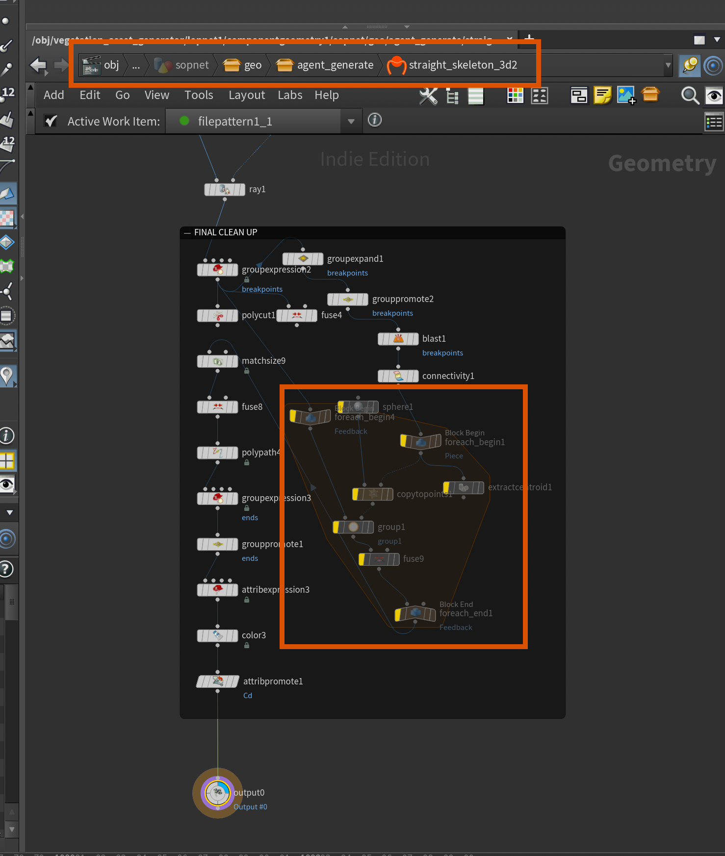
If you right click on the node and choose Allow Editing of Contents you can dive in and go to the bottom of the included network. There you'll find a For Each network that needs to be disabled. As far as I can decipher, this section is supposed to perform some kind of cleanup, but in a lot of my skeletons, it ended up deleting the entire skeleton instead. There are probably ways to fix this, but I ended up building my own skeleton cleanup setup instead to have more control (more on that in the next section!).
With that disabled, you should get a nice and precise skeleton based on your input mesh.. The only setting I changed in the Labs Straight Skeleton 3D node was the Fuse Distance which I set to 0.05. Although this will depend on your model scale.
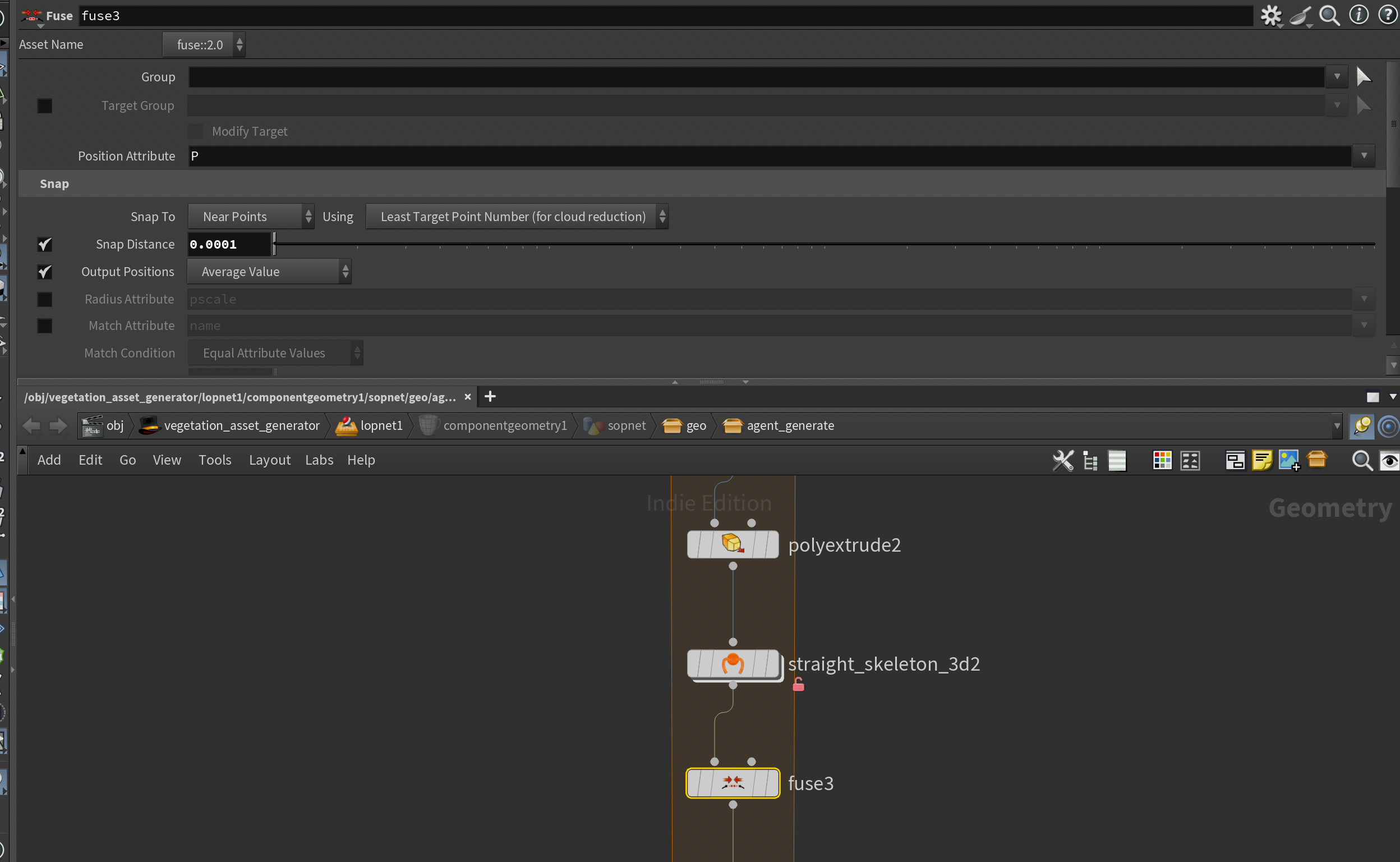
After the Labs Straight Skeleton 3D I attached a Fuse node with a very low snap distance to make sure that any overlapping points are connected.
After that, I defined an additional root joint placed at the origin using a wrangle set to run over Detail. This snippet simply adds a point/joint at the origin, and connects that joint to the closest point in the skeleton.
int root = addpoint(0, {0,0,0});
int closept[] = pcfind(0, "P", {0,0,0}, 1000, 1);

addprim(0, "polyline", closept[0], root);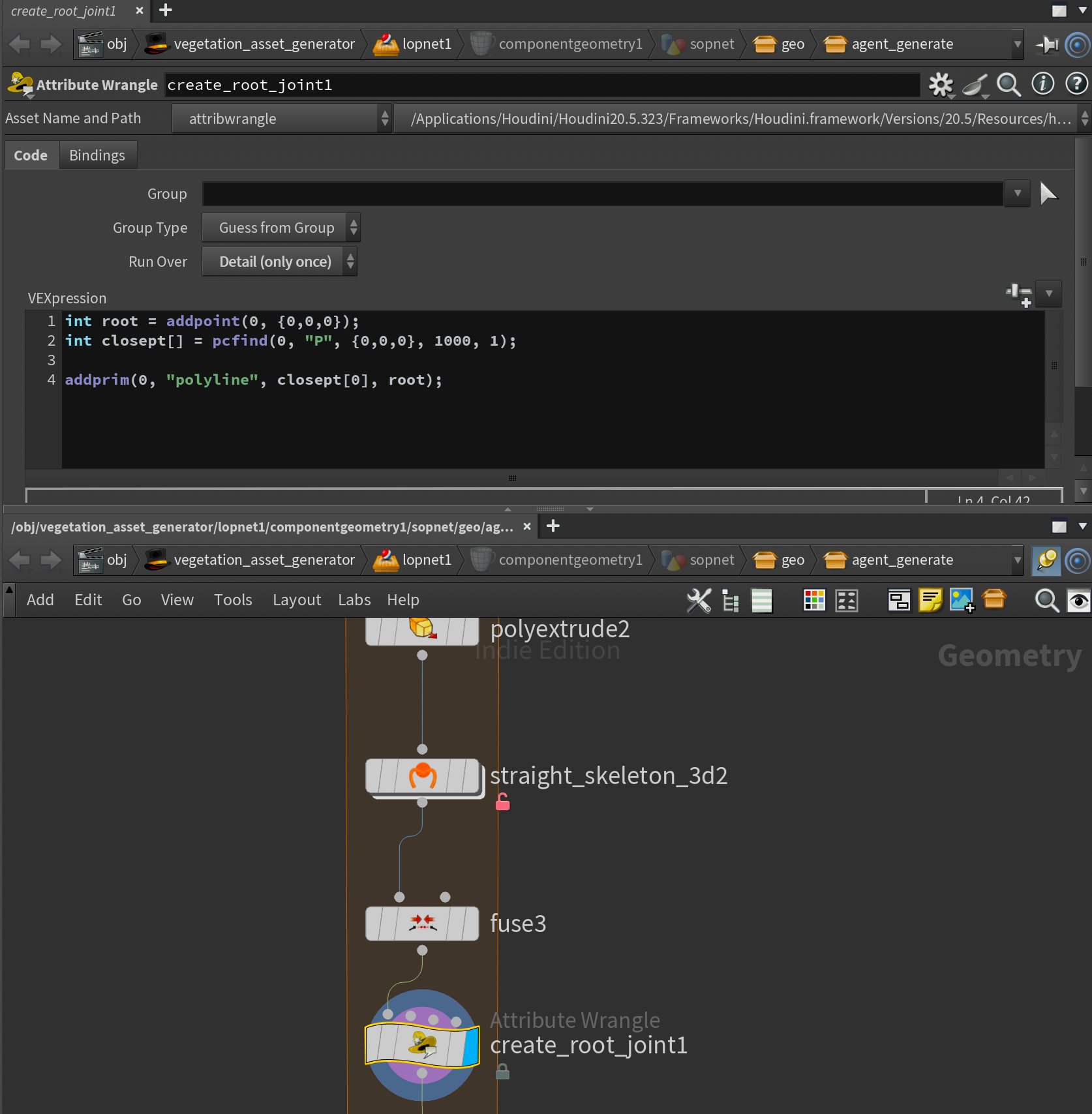
Now, if you were to connect a Rig Doctor node to this setup to initialize the skeleton you'd immediately get a warning about hierarchy cycles. While this is just a warning in the Rig Doctor node, it will actually cause our agent generation to fail, so we need to fix it. In the next section, I'll cover how to clean it up, and what hierarchy traversal cycles are.
Cleaning up Skeleton
First let's discuss why we need to clean up our skeleton in the first place. As mentioned we get a warning in the Rig Doctor . While it might not seem like an issue at first, this warning is actually what will cause our agent generation to fail once we attach an Agent from Rig node.
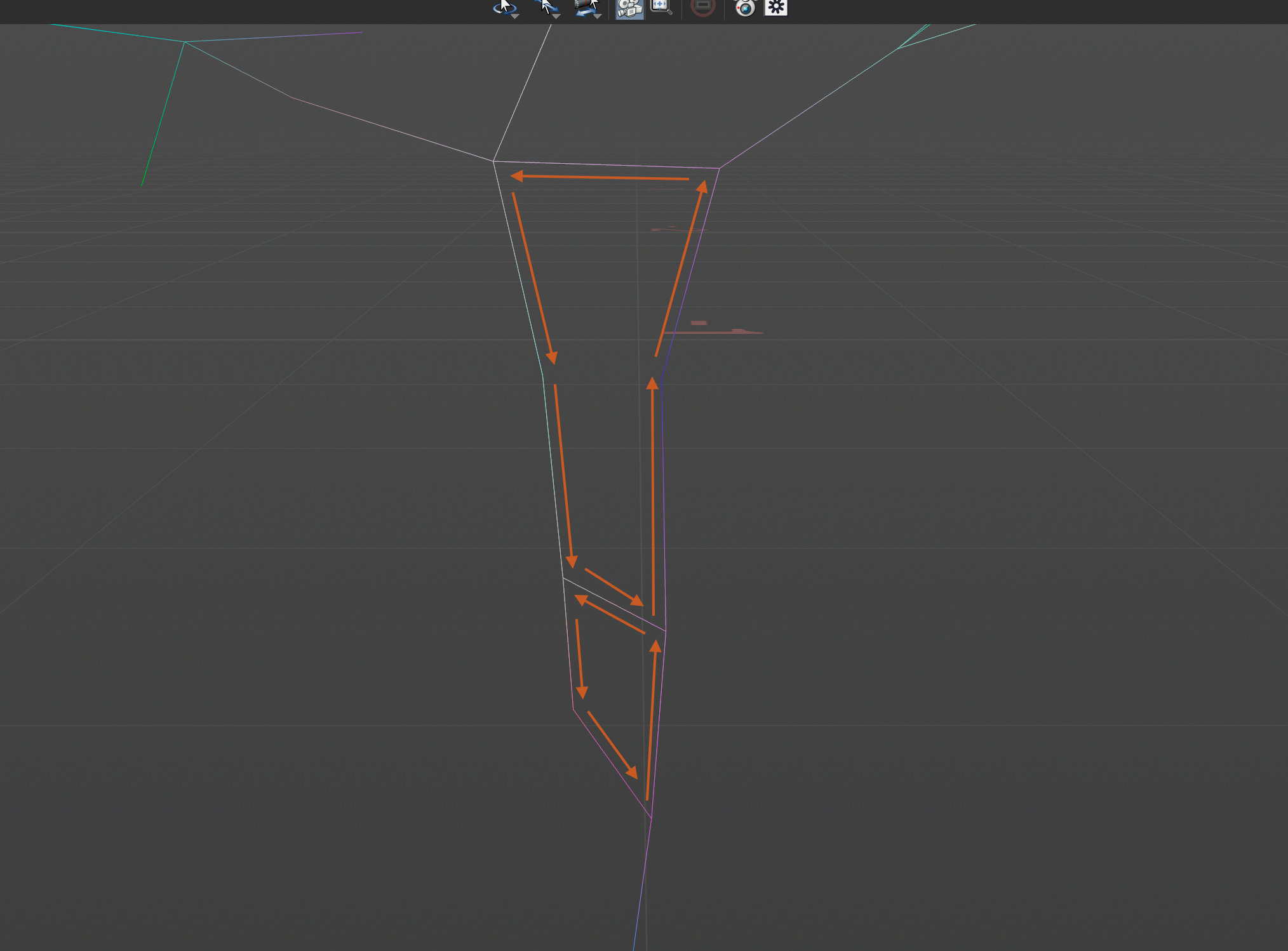
The reason it fails is because we have what's called a "Hierarchy Traversal Cycle". What this means is that one or more joint hierarchies have a parent that is also a child in the same hierarchy.
Here's a more visual example where the joints go around in a circle. You can clearly see that the joint at the stem eventually loops around to itself again - creating a cycle because it becomes a child of itself. However, it can also be less visible if the joint direction is simply facing the wrong way.
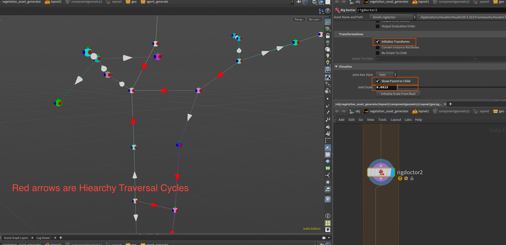
If you want to debug it yourself and see where your Hierarchy Traversal Cycles are you can attach a Rig Doctor , enable Initialize Transforms, Show Parent to Child, and lower the Joint Scale. With this you should see white and red arrows between your joints. The red arrows are the Hierarchy Traversal Cycles that we need to fix.
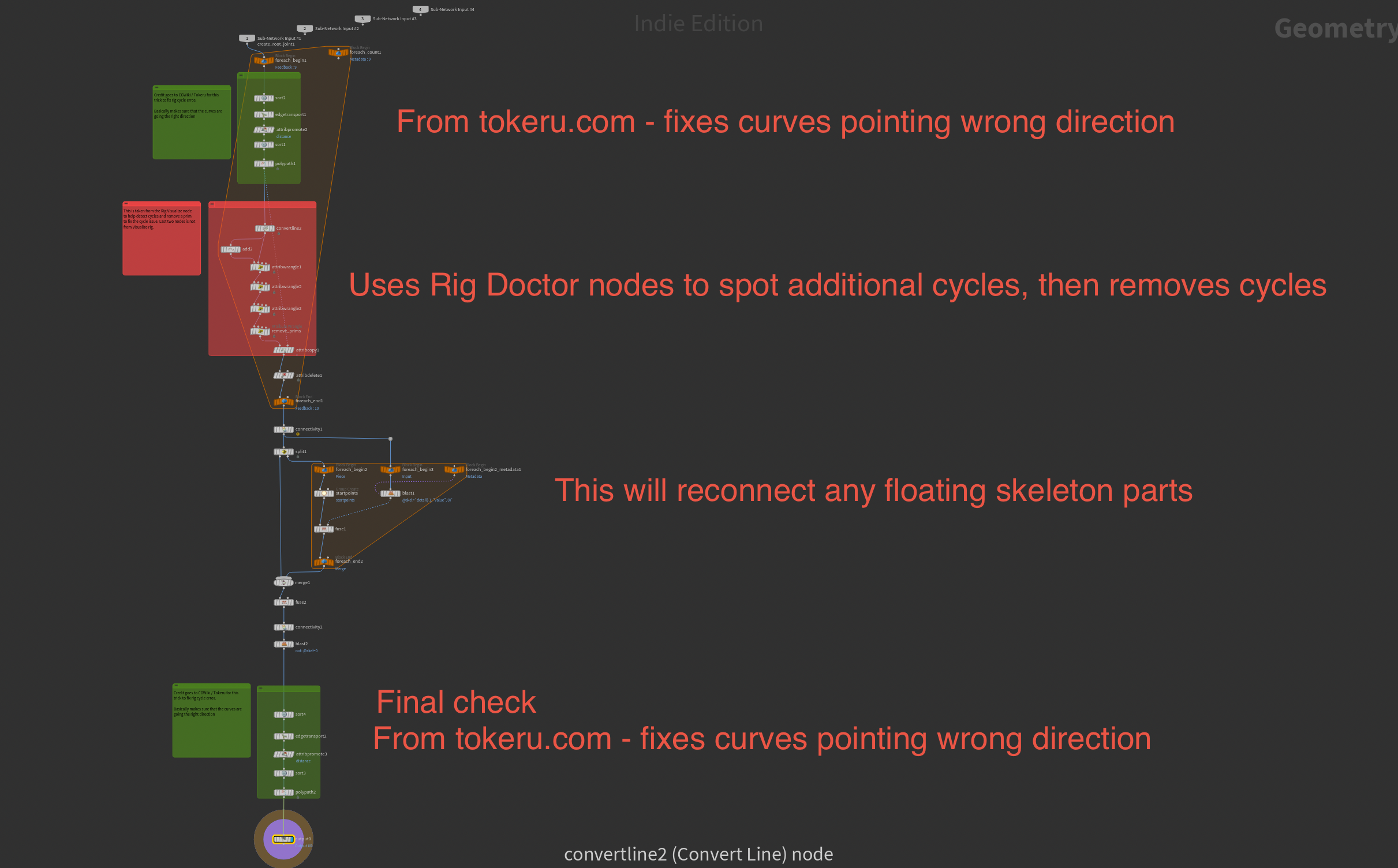
There are multiple ways to approach fixing this. In my case, I developed a custom HDA to try and catch all the different cases that might cause Hierarchy Traversal Cycles. It has worked quite well for all these plants and you can access it through my Github: https://github.com/andreask-j/akjTools (The HDA is called Fix Cycles).
I've attached a little breakdown below as there's quite a few steps to this. But essentially it starts off by fixing any curves that are pointing the wrong direction by fixing the vertex order (courtesy of https://www.tokeru.com/cgwiki/HoudiniKinefx.html ). Then I used parts of the Rig Doctor node to spot any additional cycles and remove them. I then reconnect any floating skeleton parts, and finally do a final tech check fixing any remaining curves pointing the wrong direction.
With that applied, we should have a clean skeleton ready to use for agent generation.
Rig Doctor
Finally, in order to initialize our skeleton, we need to append a Rig Doctor node. This will initialize our curves and generate a proper skeleton with initial transforms, orients, and naming.
In order to help differentiate the skeleton joints later on, I also decided to prefix each joint with the number of the current iteration in our for-loop.
To do this, go to the Block Begin (foreach_begin) of your for-loop and click Create Meta Import Node. If you're unfamiliar, this will give you an additional node you can reference for data about the current iteration of the for-loop.
Back in the Rig Doctor node you can click the little wheel in the top right corner and Add spare input to reference the Meta Import node. I find this a little easier than having to write the full path to the node when we need to reference something (with spare input you can use -1 instead).
Then, to create unique joint names, write point_detail(-1, "iteration", 0)_ in the Prefix parameter to prefix the iteration number to the joint name. Finally, enable Initialize Transforms and Re-Orient To Child to initialize transforms and joint orientations.
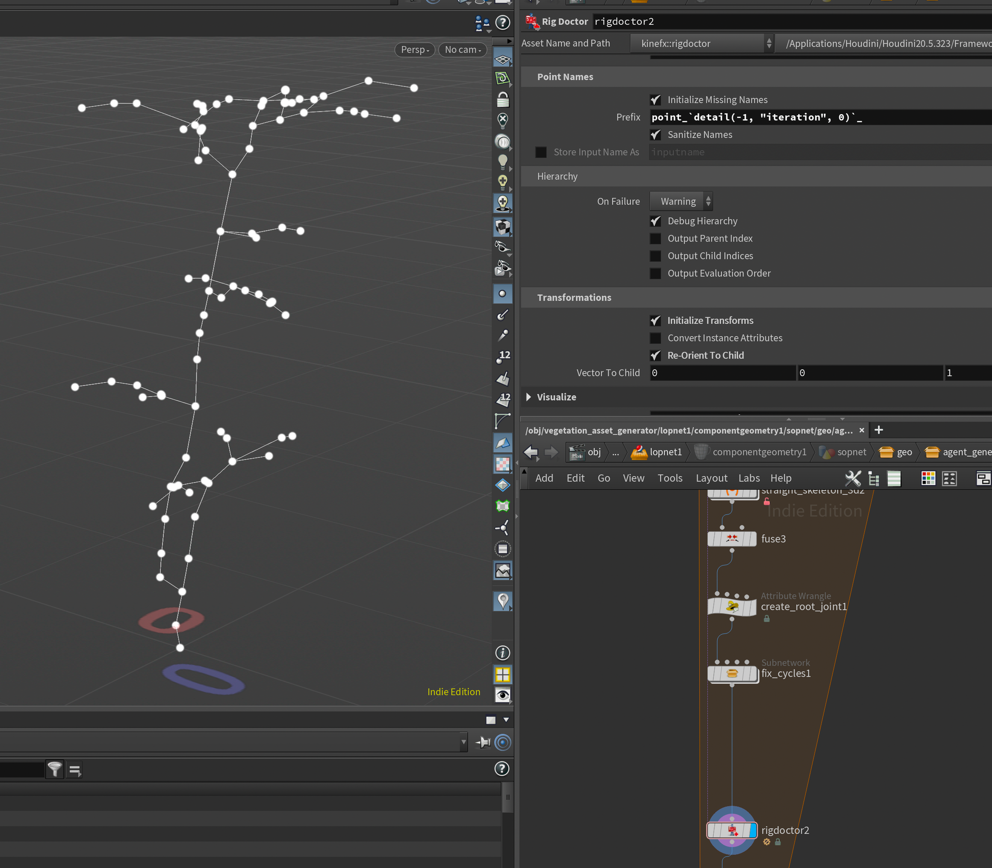
If the previous steps have been completed correctly you should now have a clean skeleton with no warnings on the Rig Doctor node.
Skinning
Skinning continues to be the weakest point of this setup. It was quite hard to find an automatic skinning setup that worked on all inputs. And sometimes I would also encounter errors on the skinning nodes.
I ended up simulating a sort of "Try Except"workflow where I try to use the most "precise" skinning operation first, then try a less precise one if that fails, and finally if that one fails, try the simplest skinning operation. This way we always end up with some sort of skinning on the vegetation, with priority on the most precise setups. All skinning setups have the same inputs - first input being the original unpacked geometry, second and third being the output from the rig doctor.
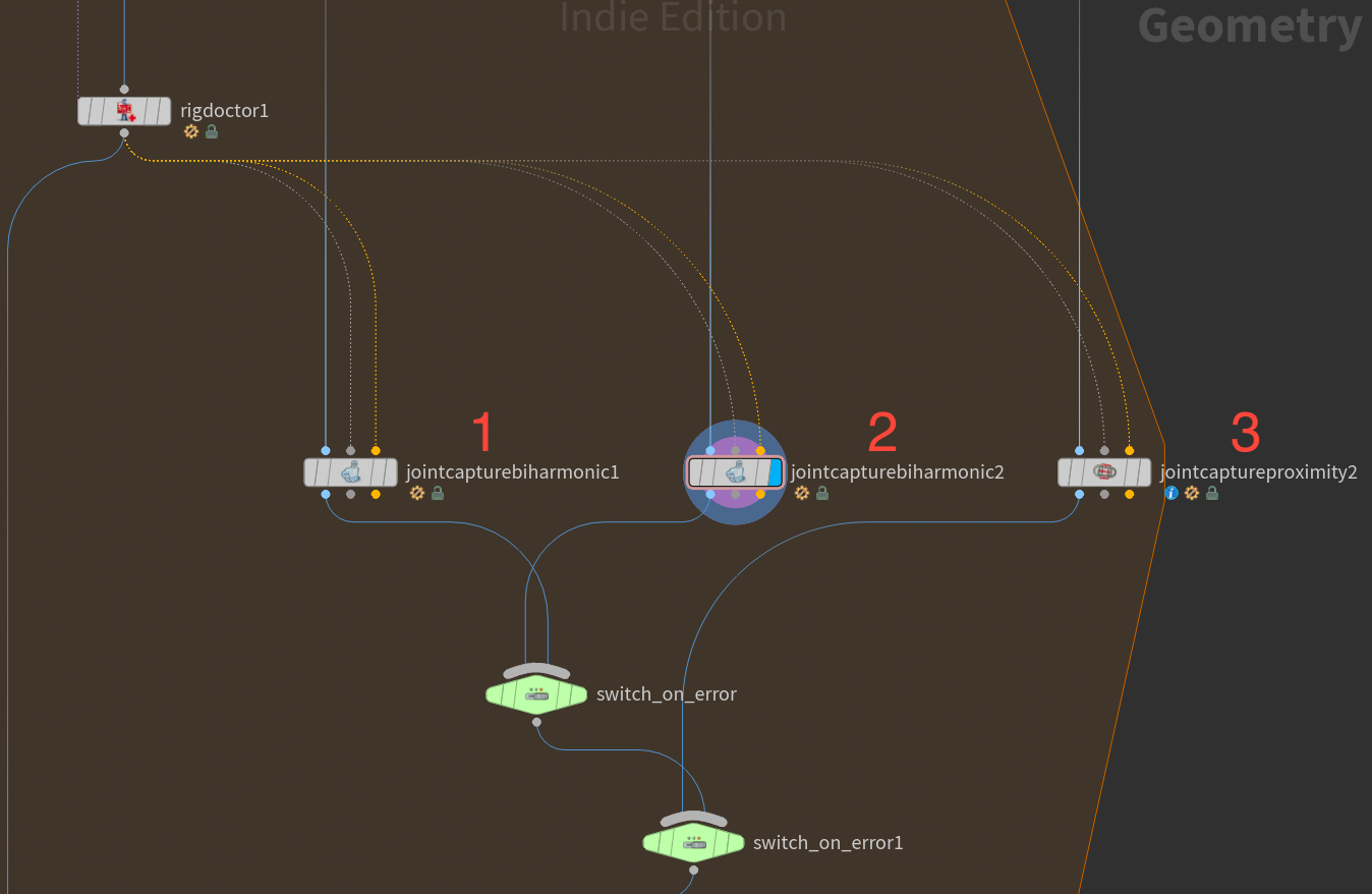
First attempt is a Joint Capture Biharmonic set to Exact.
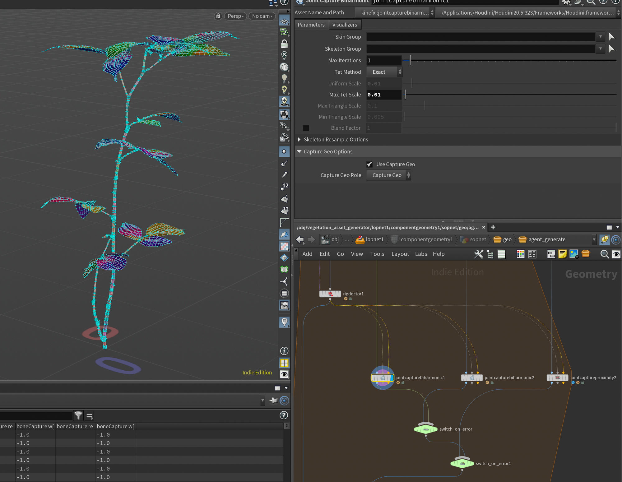
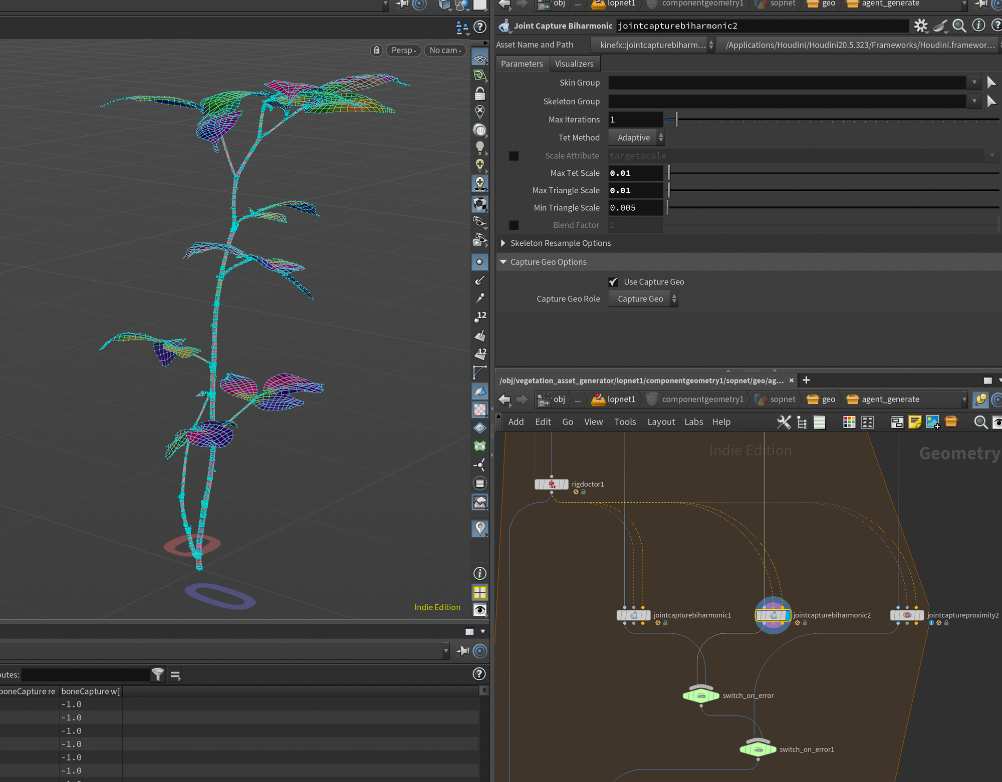
Second attempt is another Joint Capture Biharmonic set to Adaptive.
And finally, the third attempt which should always work but is less nice. A Joint Capture Proximity.
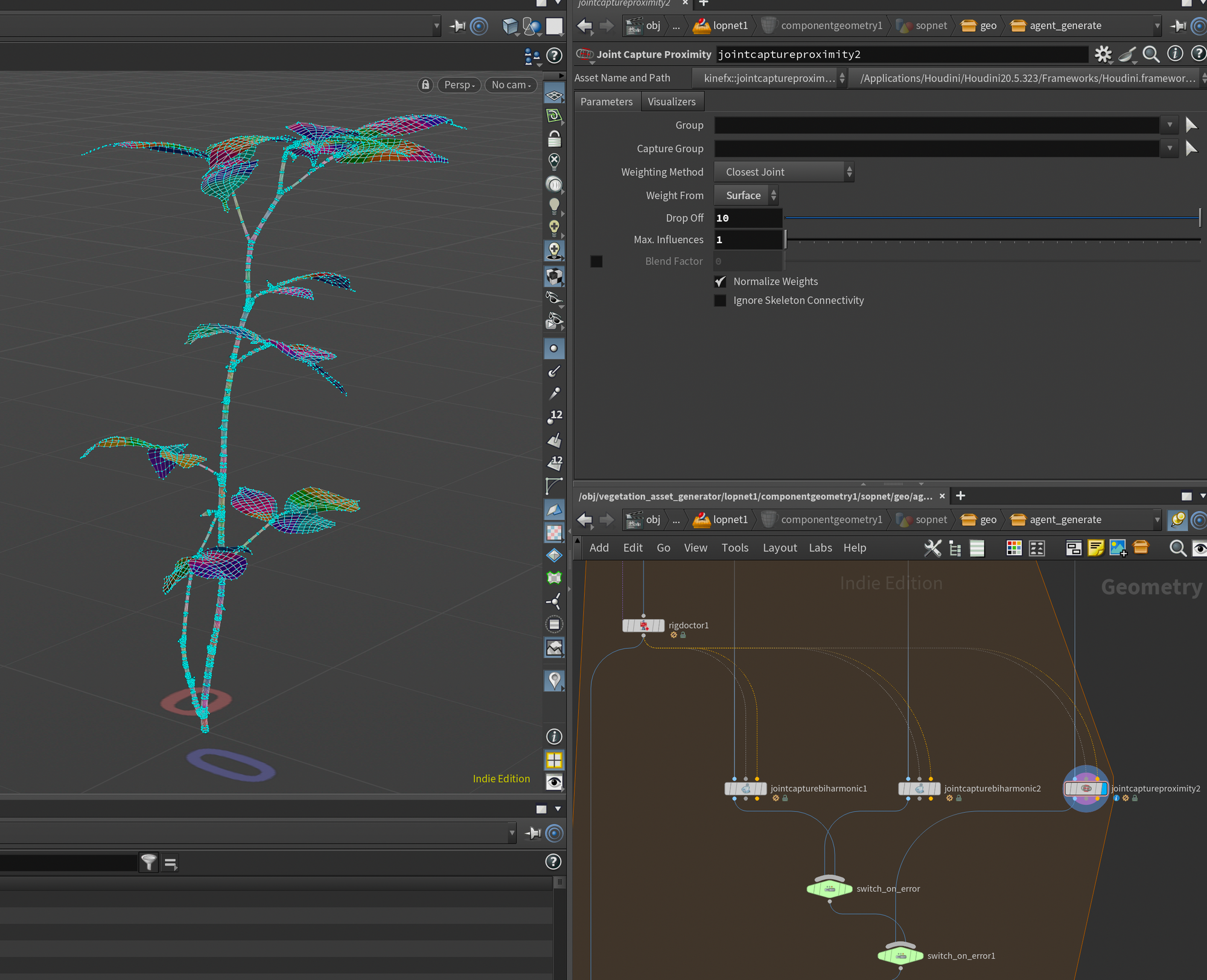
The way I check for errors is using a Switch node that checks if the second input has any geometry. If not, it will try the next one, and so forth. The code in the switch nodes is the following python script:
if(hou.pwd().inputs()[1].geometry()):
    return 1
else:
    return 0
Code for Switch node to check for errors / no geometry.
Initializing Agents
We've now reached the final part of our agent setup. At this point, we simply need to set up the actual agents, attach our geometry as an agent layer, and name our agents for LOPs.
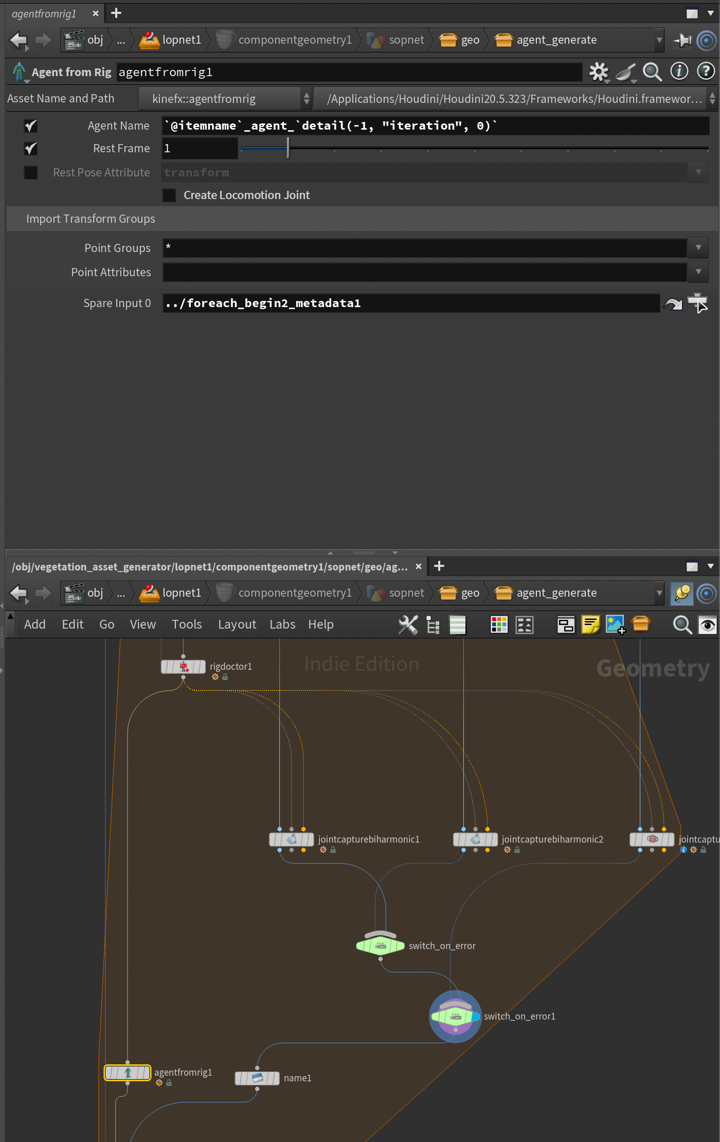
Add an Agent From Rig SOP and plug the output of the Rig Doctor directly into it. This will initialize our skeleton as an agent. Keep in mind that if the skeleton cleanup we did earlier failed, you would likely get an error now.
Like before, I also adde a spare input to the Agent From Rig and connect the Foreach Begin Metadata node to it. This will help us name our agent.
Set the Agent Name parameter to:
`@itemname`_agent_`detail(-1, "iteration", 0)`And disable Create Locomotion Joint (this is mostly for when you're doing actual crowd animation and won't apply to this setup, so we can disable it).
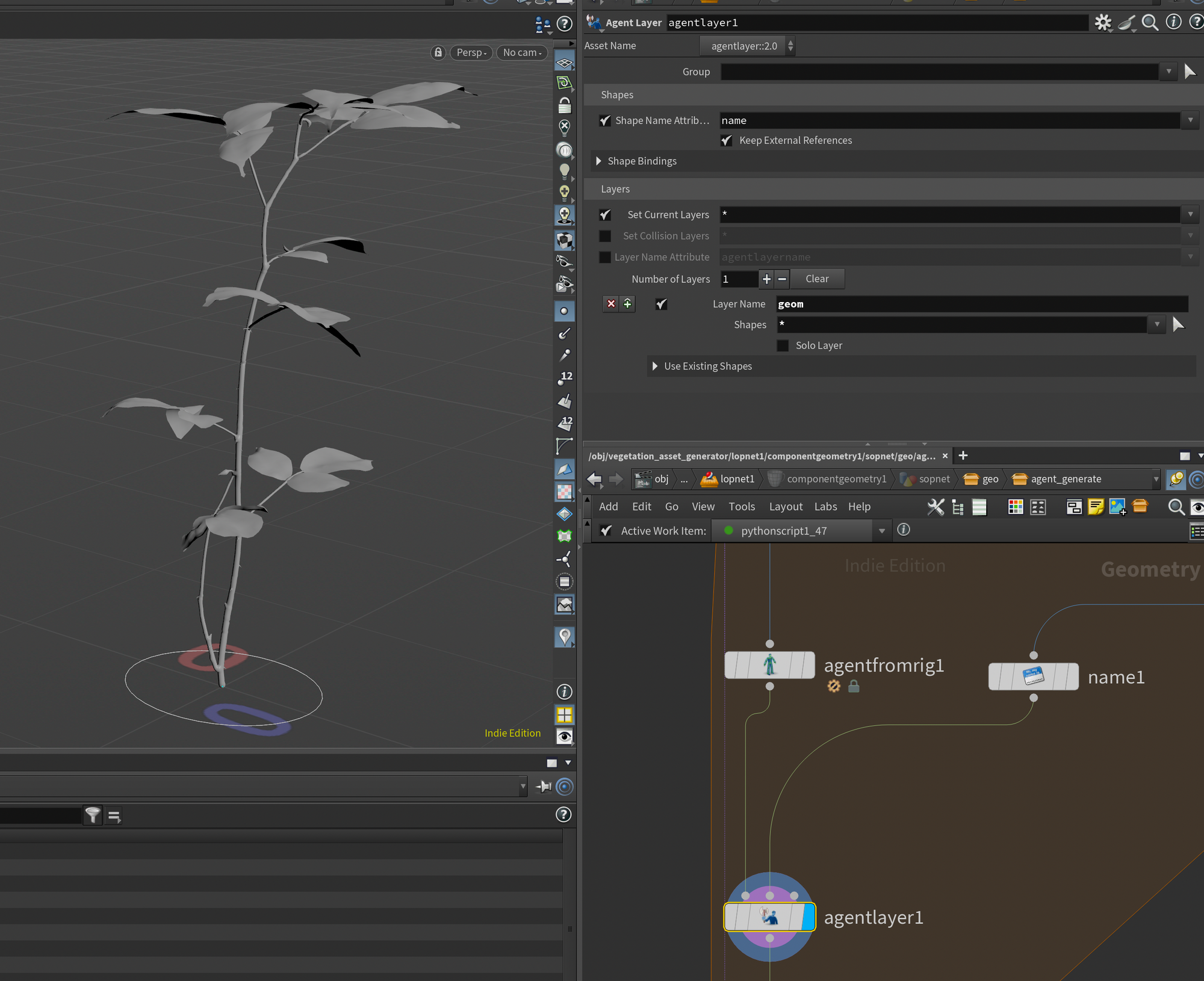
@itemname variable in the Agent Name - this is a variable we'll set up in the next step in TOPs/PDG to allow us to grab the name of the vegetation asset.Now we need to attach our geometry to our agent. This is done using an Agent Layer node. Before we do that I also name our geometry using a Name node and simply call it geom . This allows us a bit more control of the naming in LOPs.
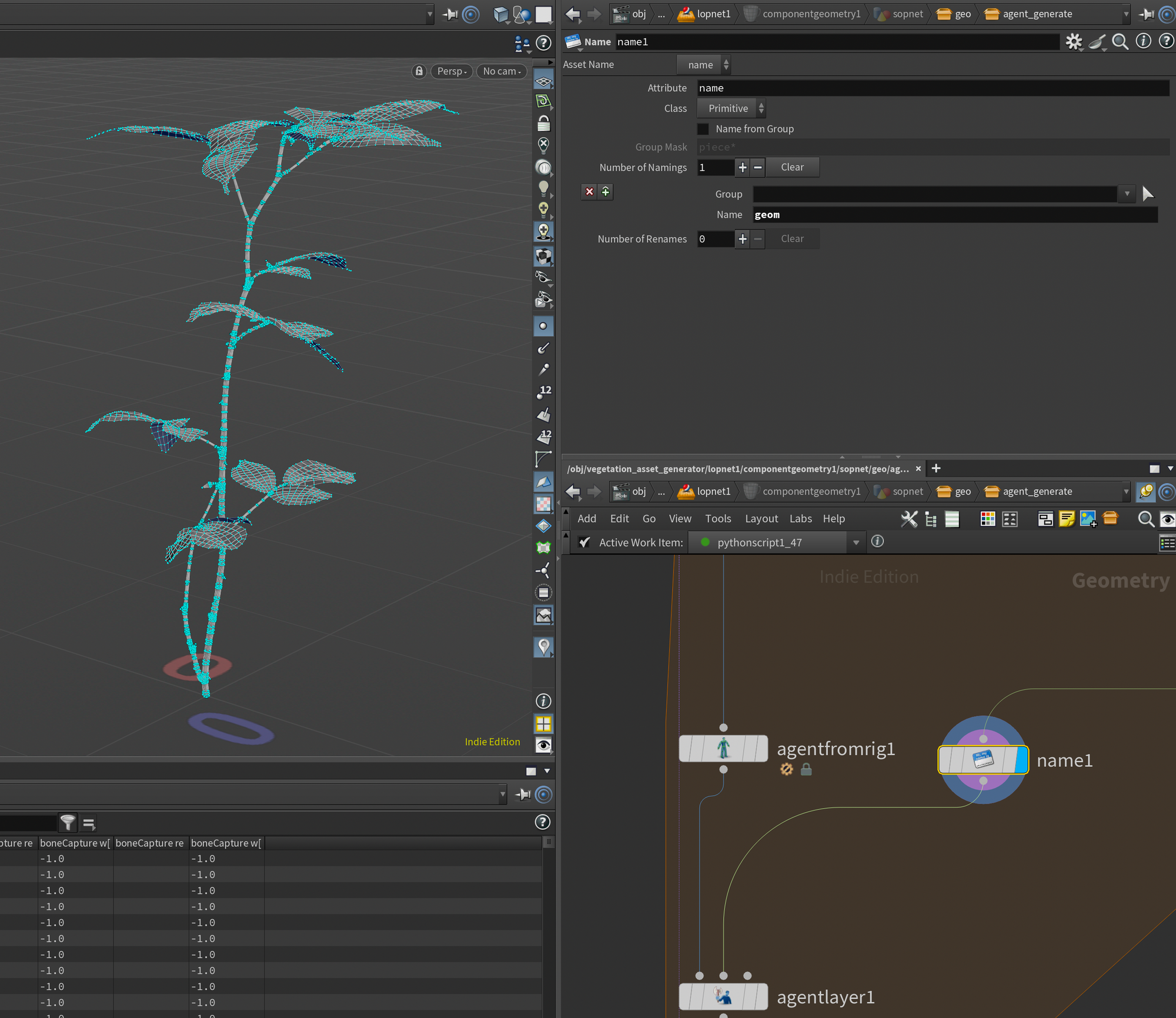
Plug the output of the Name node into the second input of the Agent Layer, and the Agent From Rig into the first input. Nothing too major in terms of settings here, I just named the layer geomin here for consistency.
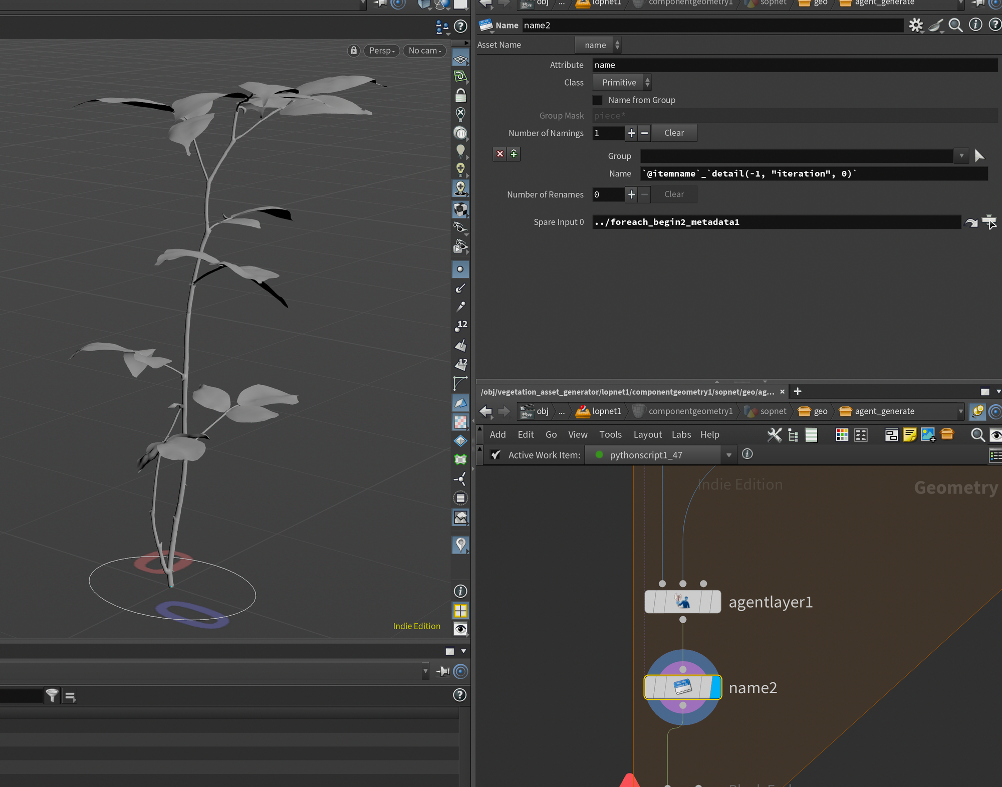
Finally, in order to get a clean resulting naming in LOPs I added a final Name node, added the Foreach Begin Metadata node into a spare input, and set the Name to the same as our agent name above.
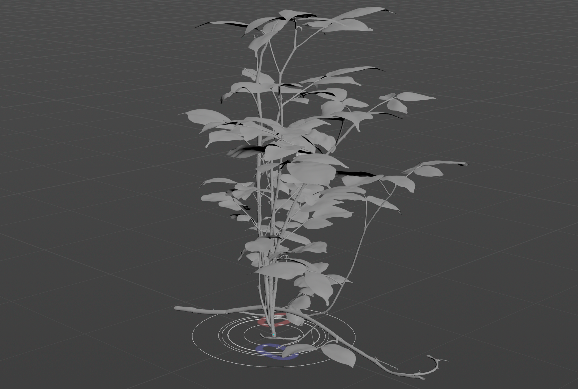
And that's it for agent generation! Now you can disable Single Pass on the For-Each End node so we can cook all the vegetation in the currently selected TOPs work item. It should look something like this - you can see we get an agent for each model.
In order to get the @itemname to work, we need to add a little Python node in TOPs to initialize this custom variable. So, go back to TOPs and add a Python Script node with the following code:
itemname_list = work_item.stringAttribute("filename").split("_")[0:3]
work_item.setStringAttrib("itemname", "_".join(itemname_list))

outputdir = work_item.stringAttribute("directory").split("/")[0:-1]
outputdir.append("usd")
work_item.setStringAttrib("outputdir", "/".join(outputdir))

texture_prefix = work_item.stringAttribute("filename").split("_")[0:2]
work_item.setStringAttrib("textureprefix", "_".join(texture_prefix))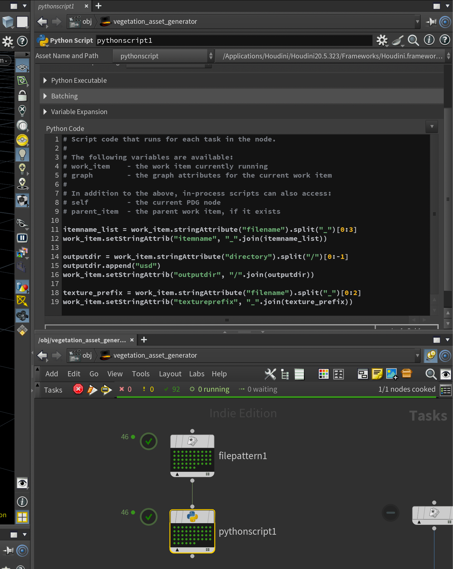
Basically, all of these variables are just extracting data from the naming of the assets to help construct texture paths, item names, etc. - this way, we can batch process entire folders of vegetation (as long as they have the same structure). If you're not using GScatter vegetation, you'll likely need to adjust this code to accommodate.
This will also add some other additional attributes that we'll be using in the next step.
Remember to cook this node by selecting the Python Script node and pressing SHIFT+V.
If you want to learn more about agents, check out my article on Crowd Generation here:
Batch USD Asset Generation
Batch-generating USD Assets using PDG complete with textures and shaders.
With our agent generator setup ready, we can proceed into Solaris and start setting up the actual USD assets. Our goal is to create a generic setup that we can use to batch-process any amount of vegetation models.
Component Geometry
First thing we need to look at is finishing the setup of our Component Geometry node. If you recall, we set up our agent generator inside this node. This will be our high-res render purpose geometry. However, we also need to set up some good proxies.
Our proxy geometry needs to go into the proxy output node inside the Component Geometry node. The first thing I did was loading each alembic in using an Alembic SOP. In the File Name parameter we once again need to use the variables generated in TOPs to access the same file as in our agent generation subnetwork. In this case I used:
`@directory`/`@itemname`_lod2_OL.abc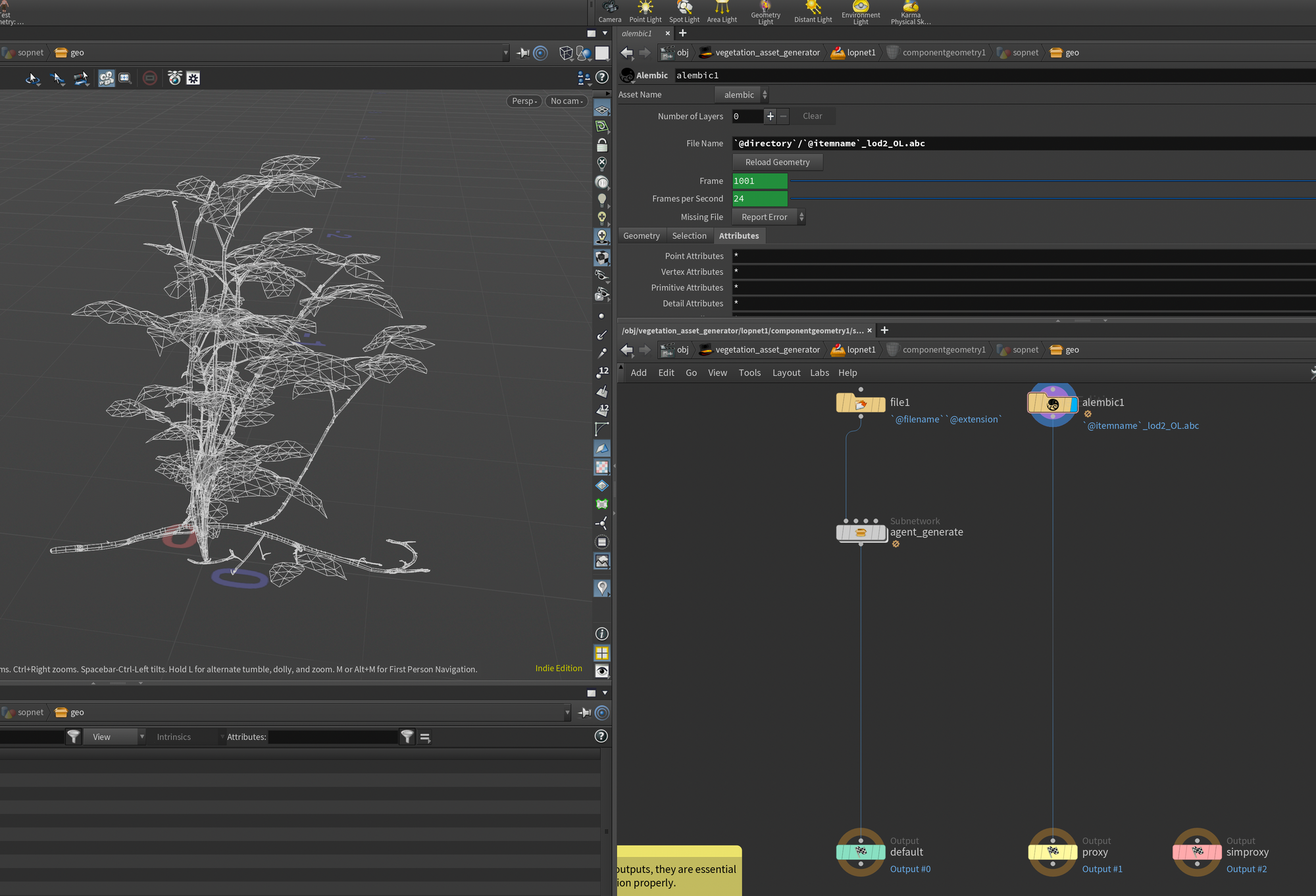
Component Geometrynode. Notice that I'm loading lod2 instead of lod0.Next, we need to setup some naming attributes to get the geometry ready for LOPs. I created a Name node set to @itemname to once again fetch the name of our current item from TOPs.
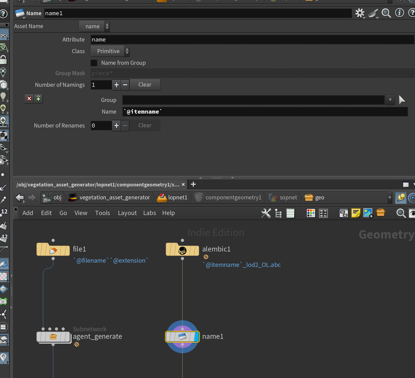
Right now however, all the meshes will have the same name. In order to fix that we need to number them the same way we did inside of the agent_generate subnetwork. In this case I did that with a small Attribute Wrangle set to run over primitives:
s@name += "_" + itoa(@primnum);This snippet adds a _ and the prim number to each current primitive - matching our agent naming.
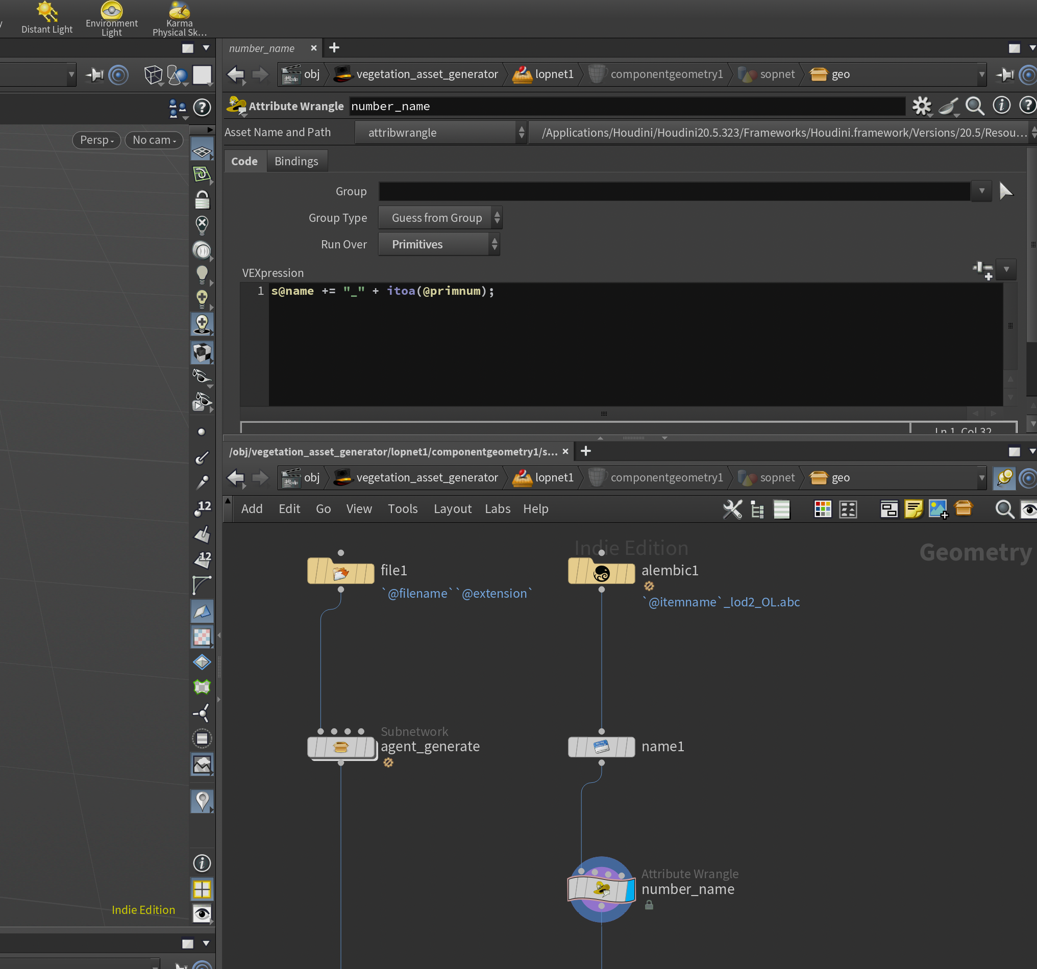
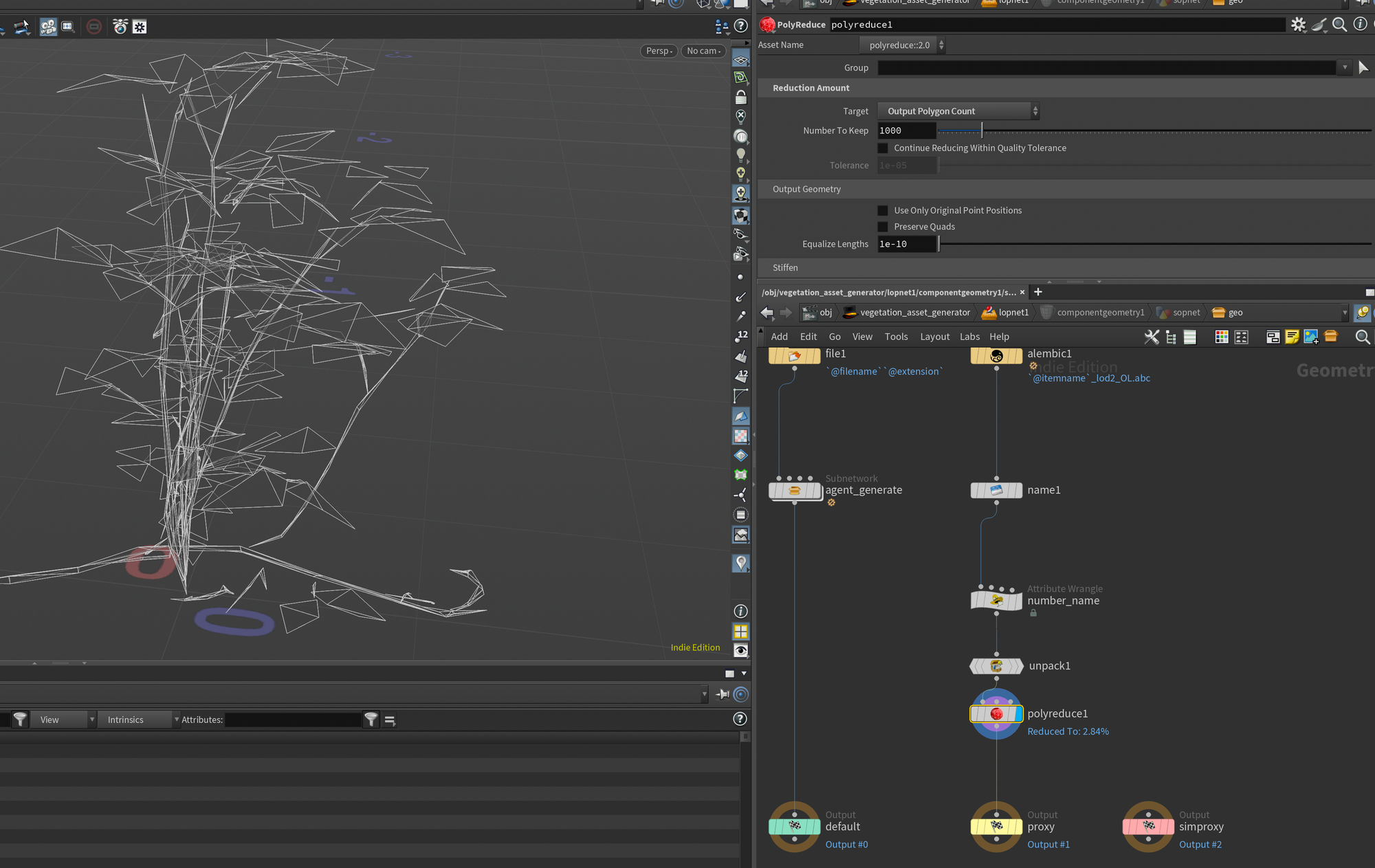
Finally, I decided to lower the resolution a bit further of our geometry for optimization's sake. First I unpacked the geometry using an Unpacknode - remembering to transfer the name attribute. And also toggling Convert Polygon Soup Primitives to Polygons (by default a lot of alembics are loaded as polygon soups which we can't modify the same way as regular geometry).
Finally I added a Poly Reduce set to a specific target polygon count. In this case I chose 1000 as I wanted all vegetation to only use that many polygons in their proxy version.
With that done our Component Geometry node should now output a proper USD stage complete with proxy geometry and agents.
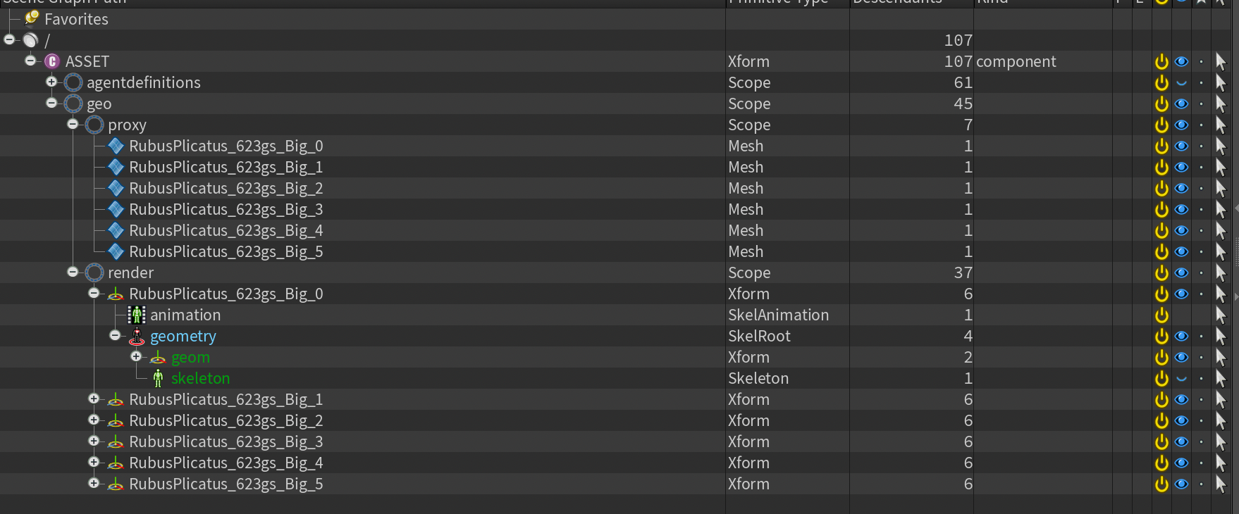
Now, if you want to be extra clean you may want to get rid of the agentdefinitions Scope - this is because by default the SOP Import treats agents like a crowd - meaning we get instances inheriting from the agent setups in the agentdefinitions Scope. In order to fix this we unfortunately need to edit the Component Geometry node and go to the base_geo node, and change Agents to Create SkelRoots instead of the default Create Instanced SkelRoots.
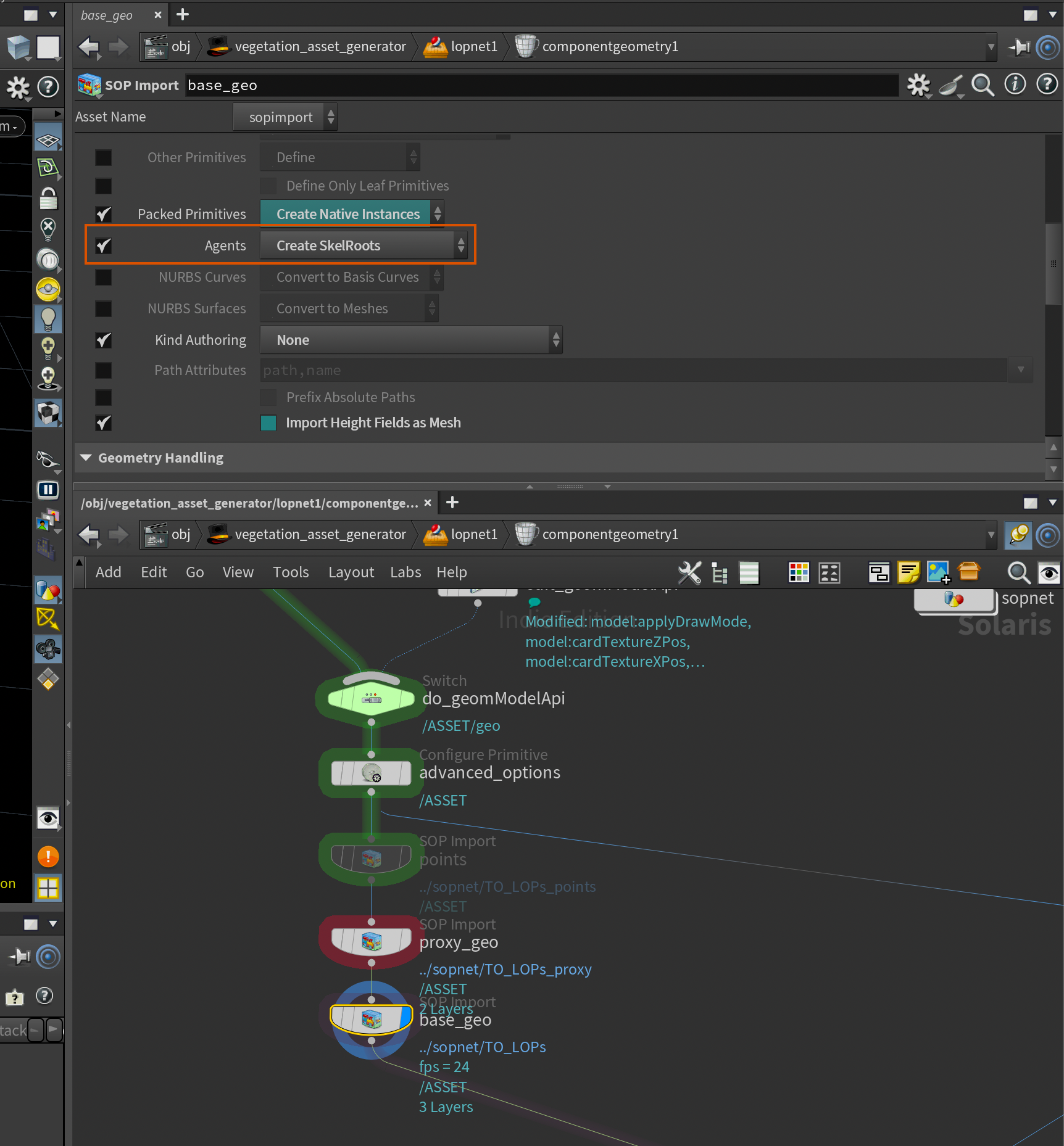
Component Geometry node.This will result in the following stage which is a bit cleaner for our use-case:
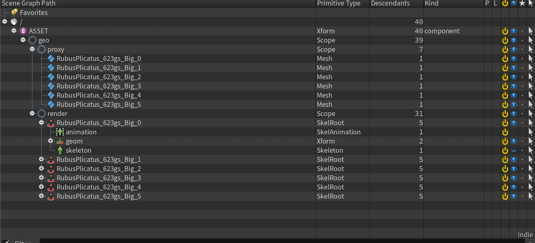
agentdefinitions.Variants
Next, we need to set up some variants. You'll notice that right now all of the different vegetations are all visible - we want to change this to only have one visible at a time. This way we can pick specific vegetation we want to use in our layout.
For this purpose I created a setup_variants subnetwork and dived inside.
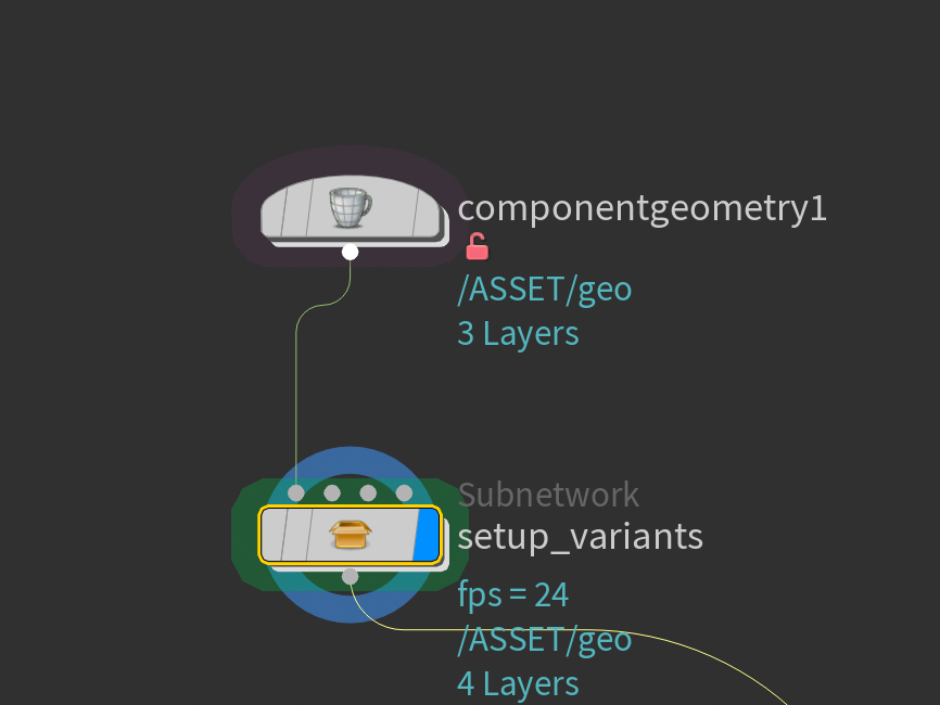
Inside the setup_variants network I created a for-each loop like you see below. The goal with this for-each loop is to take each primitive in the /ASSET/geo/render/* scope and create a variant based on each selected primitive. This is very reminiscent of how I setup variants for the assets in my other tutorial here:

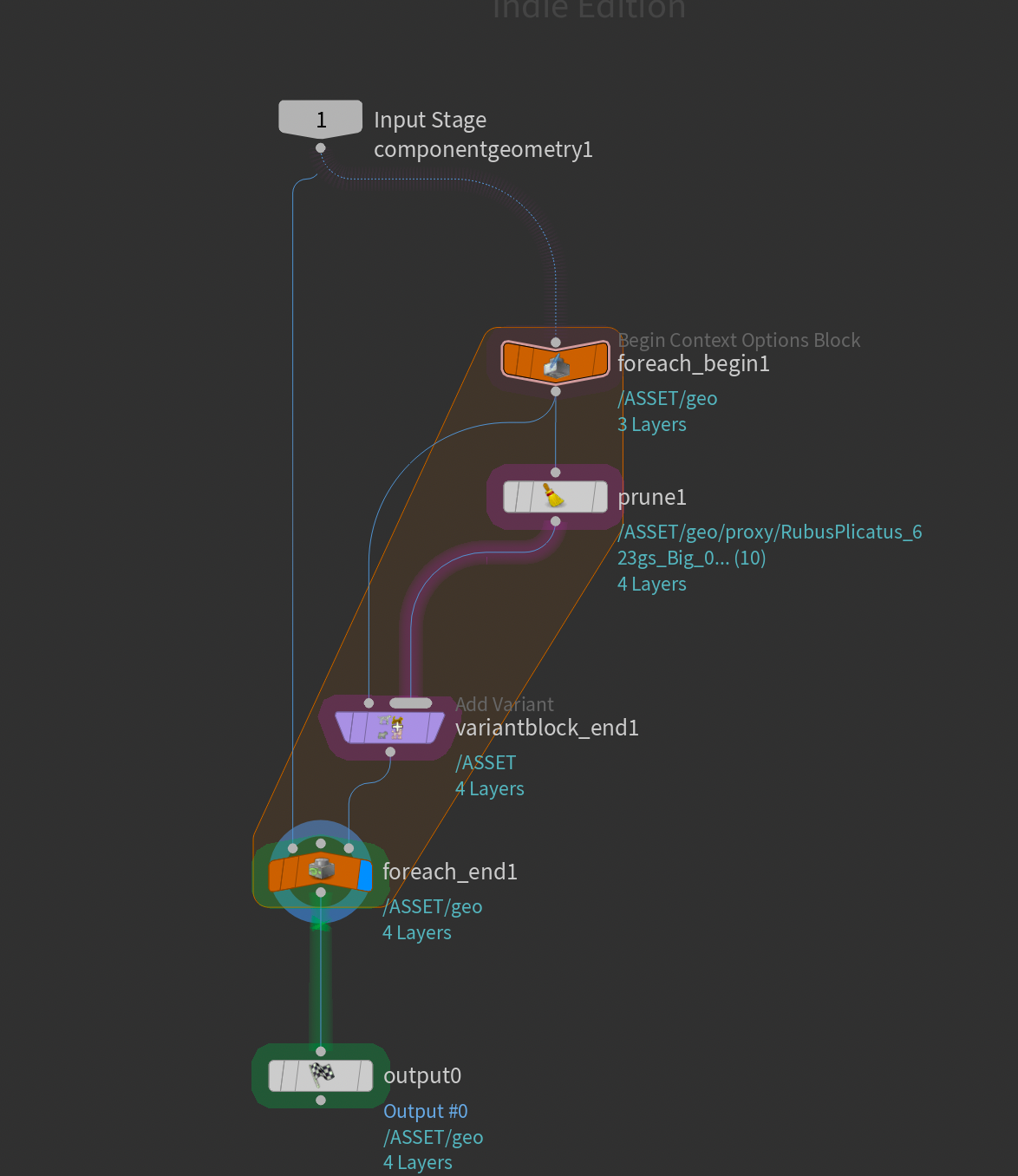
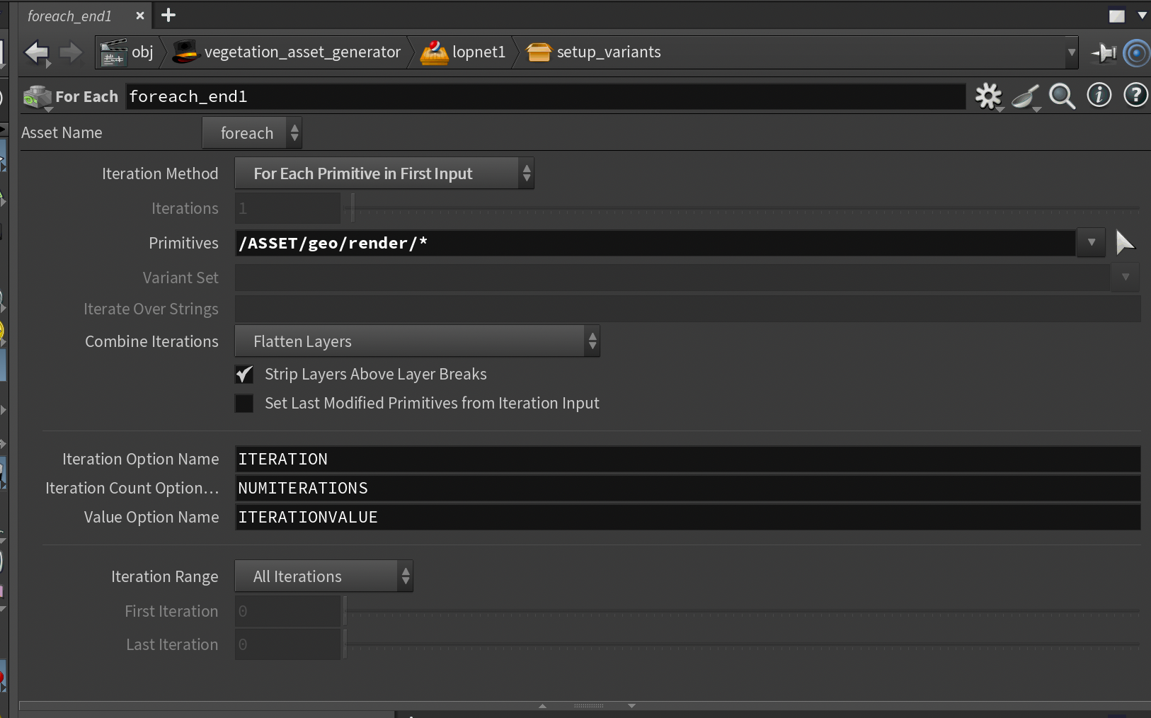
In order to do this we need to setup the foreach_end to iterate using For Each Primitive in First Input and then set the target primitives to /ASSET/geo/render/*. This will enable the foreach loop to run over each primitive in the render scope (so each agent essentially).
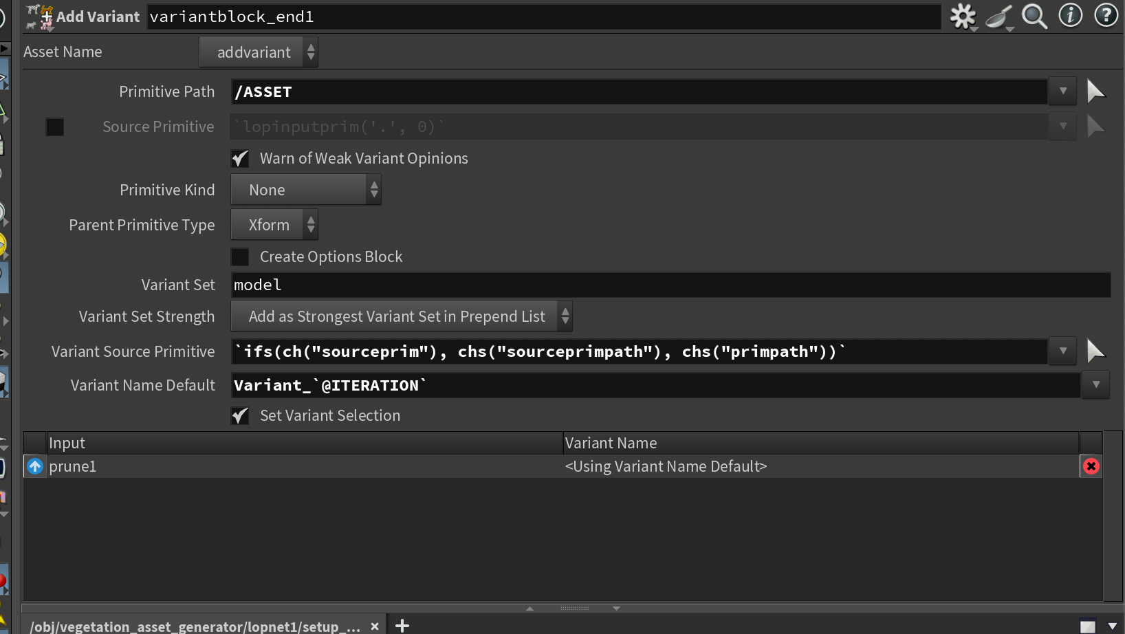
Next, in the variantblock_end (created from tab-menu with Add Variants to Existing Primitive) we first need to disable the Create Options block and delete the variantblock_begin node. Then, we need to set the Primitive Path to /ASSET since we want to target the top primitive that the Component Geometry node generates (we want to be able to select our variant from this prim).
For the variant name I also changed this to:
Variant_`@ITERATION`Which will number our variants for us. @ITERATION is a special context option generated by the foreach loop that specifies the number of the current iteration.
Finally, we have the Prune node. This will isolate only the primitives that we want for our current variation. Set the Method to Deactivate and add two Target Rules set to the following:
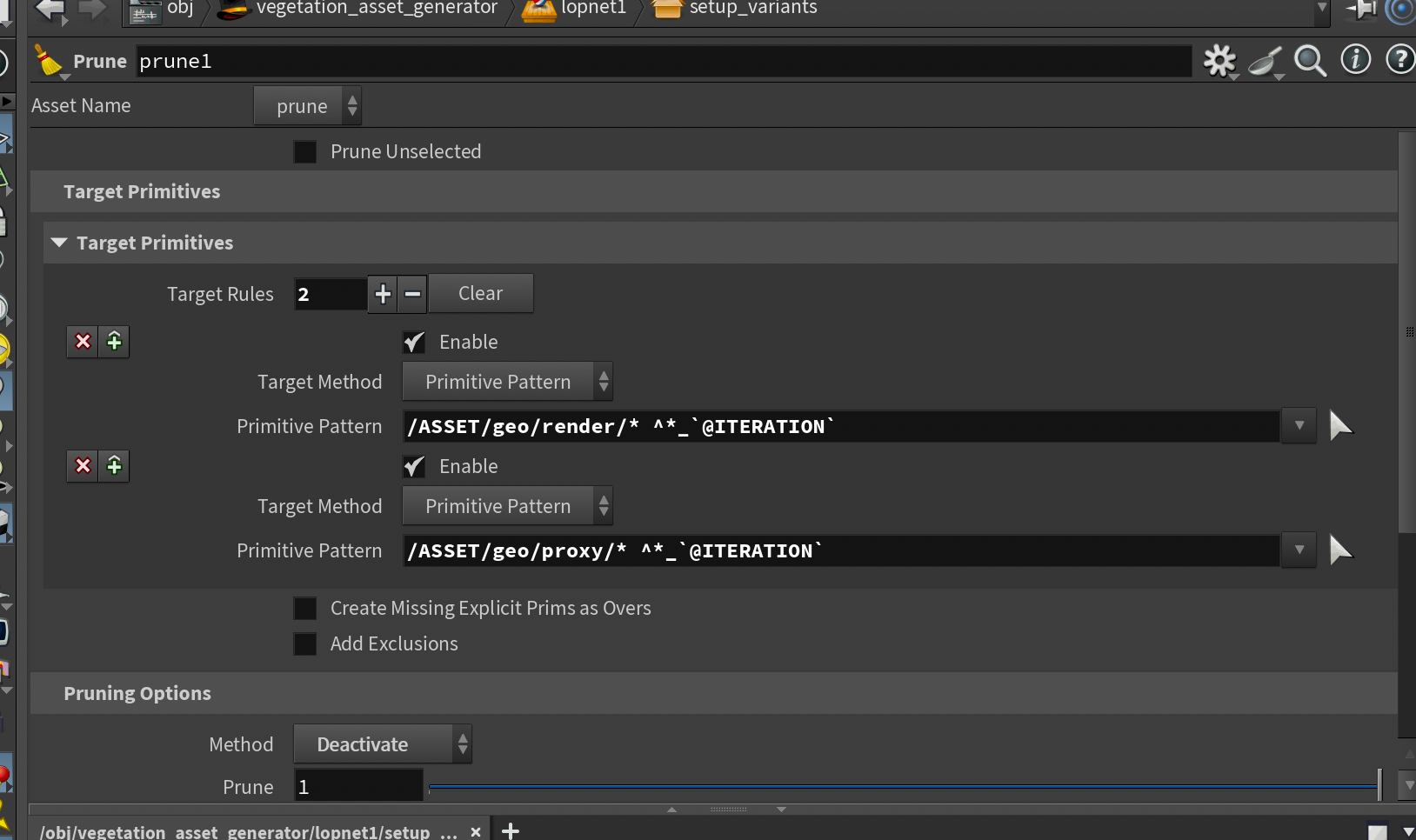
This way, the variant will work on both the proxy and render geometry. With that done, we now have working variants you can set by targeting the top primitive in the USD stage.
Mipmapping textures
Before we get started with our shaders, I want to do a little bit of preprocessing on our textures. Usually, when you download textures from the web, you won't get them mipmapped. Mipmapped essentially means that the same texture is stored in multiple resolutions in the same file. For supported render engines (most of them these days), the render engine will then swap to the appropriate texture resolution based on camera distance and render resolution. This helps keep memory and render times lower.
Most render engines these days do mipmapping on all textures automatically at render time (this is why you might sometimes find .rat files in your asset directory if you've been rendering non-mipmapped images).
However, if you want to save yourself some overhead, I recommend pre-processing your textures so they're already mipmapped before you hit render.
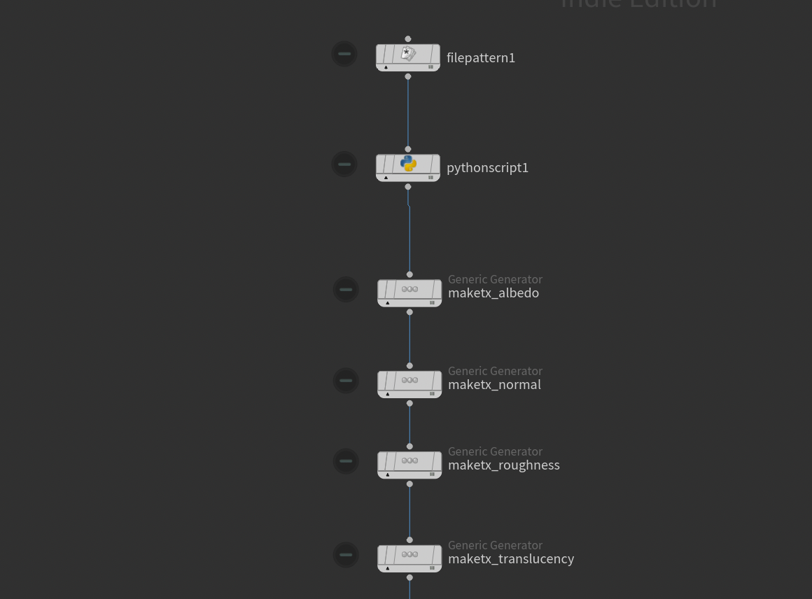
In order to do this we'll attach 4 Generic Generators back in our TOPs network. Each of these will be responsible for processing the corresponding map for each vegetation asset. The Generic Generators in TOPs are generally just used to run a custom terminal command - in our case imaketx which is a built-in command line tool for generating mipmapped textures. It's the same one that Karma runs anytime it detects non-mipmapped textures in your render.
They mostly contain the same command, just swapping the name of the texture map. I've listed all the commands I used in my case below - you should be able to use the same if you're using vegetation from GScatter.
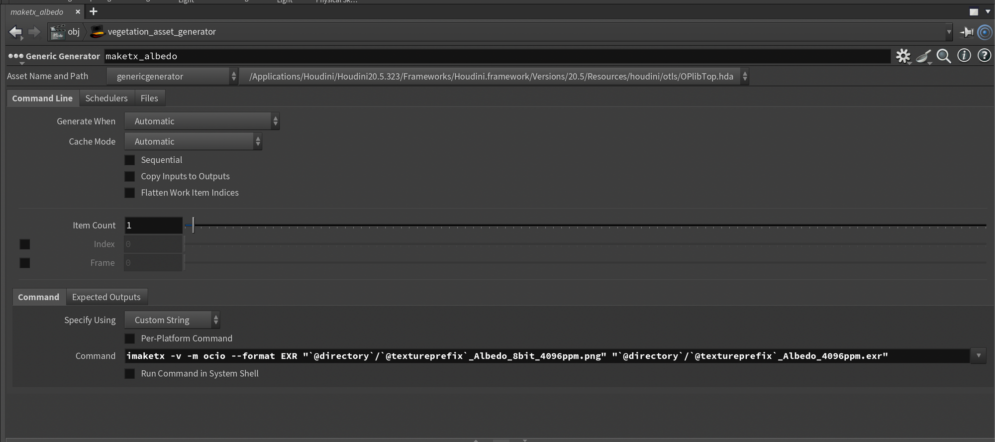
imaketx -v -m ocio --format EXR "`@directory`/`@textureprefix`_Albedo_8bit_4096ppm.png" "`@directory`/`@textureprefix`_Albedo_4096ppm.exr"Albedo
imaketx -v -m ocio --format EXR "`@directory`/`@textureprefix`_NormalOpenGL_8bit_4096ppm.png" "`@directory`/`@textureprefix`_NormalOpenGL_4096ppm.exr"Normal
imaketx -v -m ocio --format EXR "`@directory`/`@textureprefix`_Roughness_8bit_4096ppm.png" "`@directory`/`@textureprefix`_Roughness_4096ppm.exr"Roughness
imaketx -v -m ocio --format EXR "`@directory`/`@textureprefix`_Translucency_8bit_4096ppm.png" "`@directory`/`@textureprefix`_Translucency_4096ppm.exr"Translucency
Let me quickly describe how this command works and the flags I've used:
- imaketx is the name of the command that generates the mipmapped textures based on an input texture
- -v means verbose, which makes imaketx print some logging in the terminal for us (this is optional, but can be useful for debugging)
- -m is color management, which we'll set to OCIO in this case (but will depend on the color management system you use). I'm using ACES through OCIO.
- --format is the output format. Default is .rat, but I recommend using .exr as .rat is a proprietary format for Houdini and .exr works everywhere.
- Path 1 is the input texture
- Path 2 is the output texture
With all 4 nodes setup and chained together you can select the last node (in my case maketx_translucency, and press SHIFT+V to start cooking all of them. This will populate your asset directory with mipmapped textures ready to use in your shaders.
Shaders
With textures ready it's time to setup our shaders! Now we can start using the materiallibrary that was created alongside our Component Geometry in an earlier chapter.
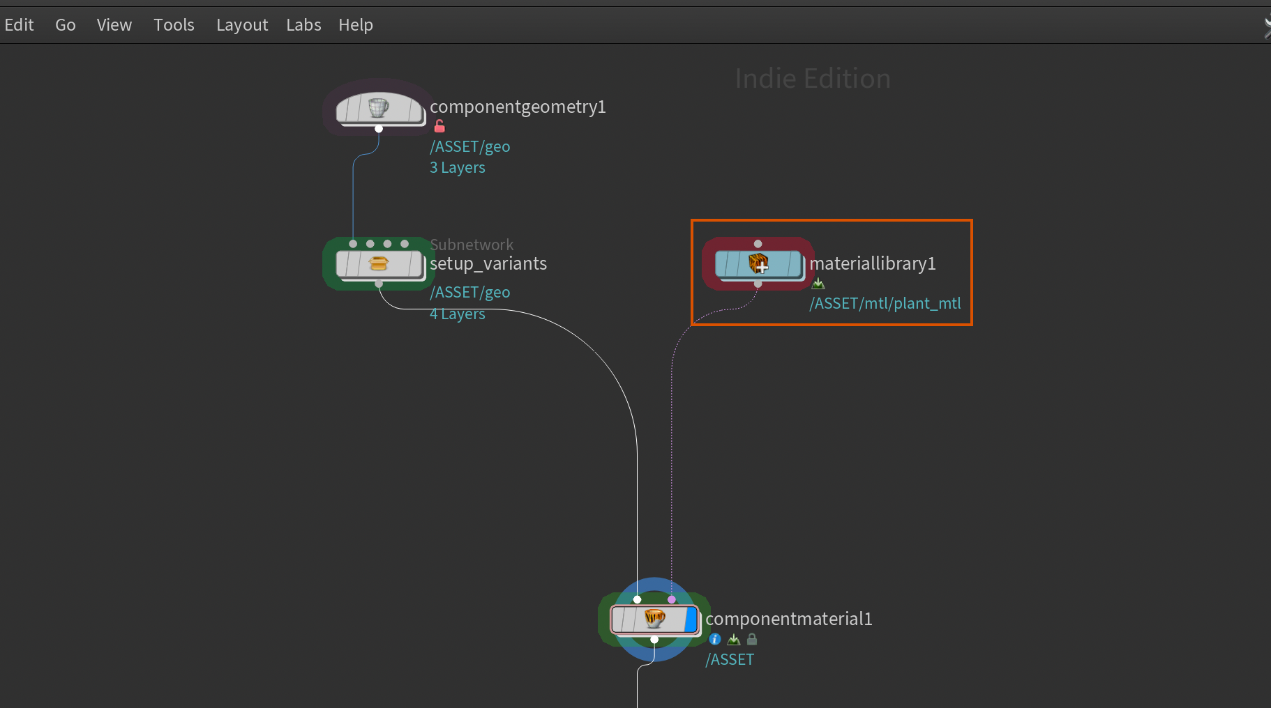
The goal here is to set up a generic vegetation shader, switching textures depending on the current TOPs work item.
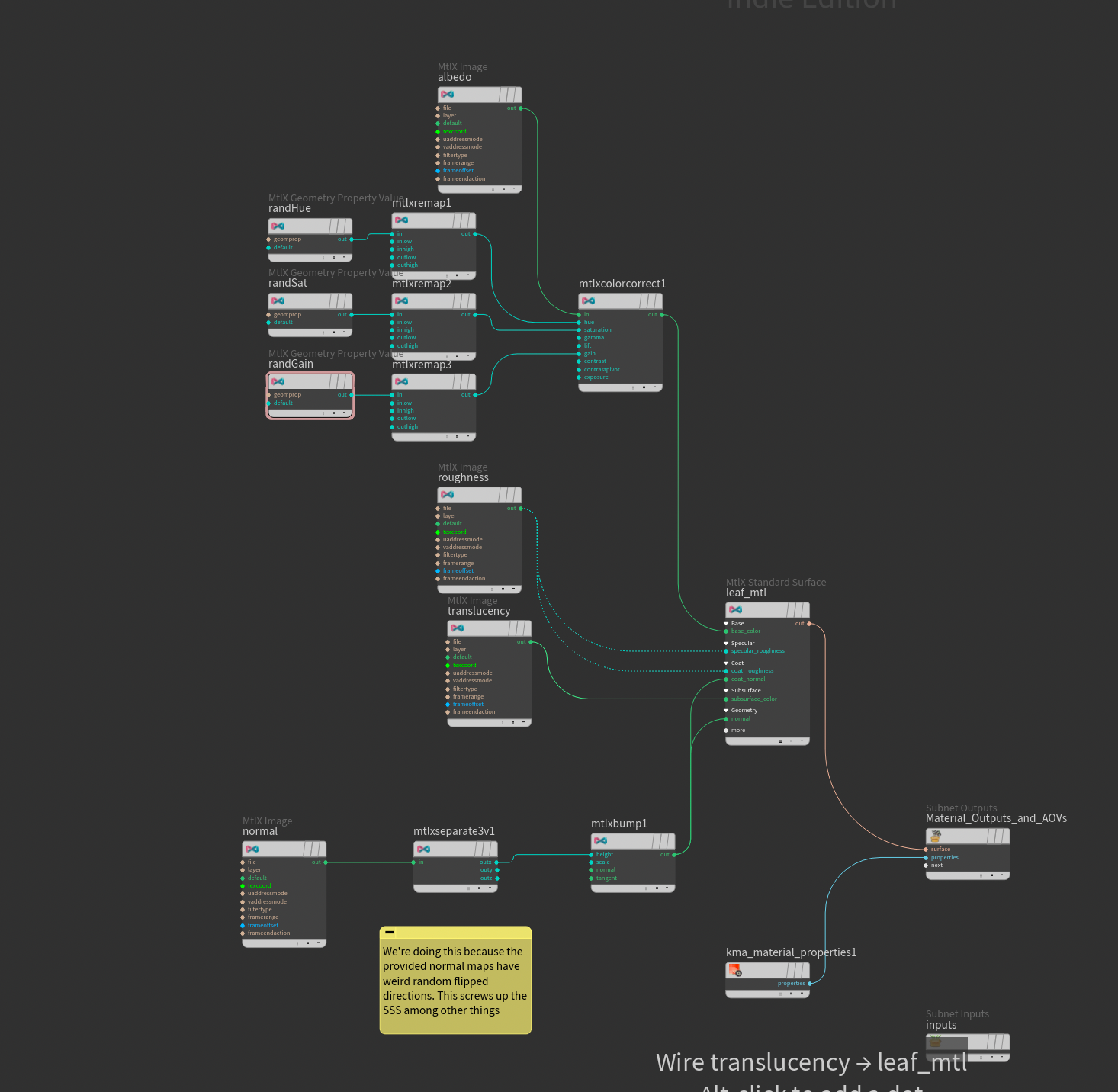
Inside the Material Library I created a plant_mtl Karma Material Builder. The shader itself is quite simple and uses the MtlX Standard Surface as our main shader. All the textures are simply plugged into the shader with a couple of minor modifications that I'll cover next.
First of all we need to make sure that the MtlX Image nodes load the texture maps corresponding to the current active asset / TOPs workitem. In order to do that we need to use our TOPs variables in the Filename of the Mtlx Image like so:
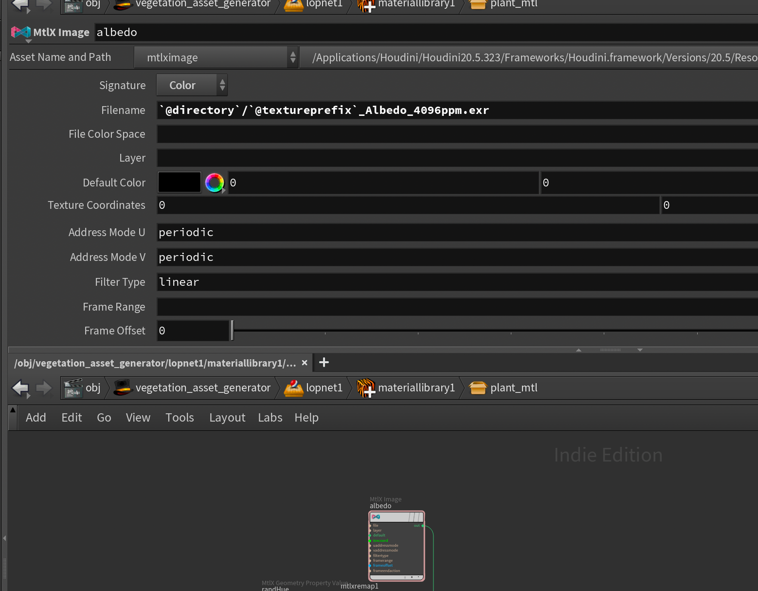
Below you'll find the Filenames I used for the various texture loaders. This will of course depend on where the assets come from, but this should work for GScatter (provided you've converted the textures to .exr in the previous step).
`@directory`/`@textureprefix`_Albedo_4096ppm.exr`@directory`/`@textureprefix`_Roughness_4096ppm.exr`@directory`/`@textureprefix`_Translucency_4096ppm.exr`@directory`/`@textureprefix`_NormalOpenGL_4096ppm.exrThese MtlX Image nodes are all plugged into the corresponding inputs of the MtlX Standard Surface.
Now, there are two slight modifications I'm making in the material setup.
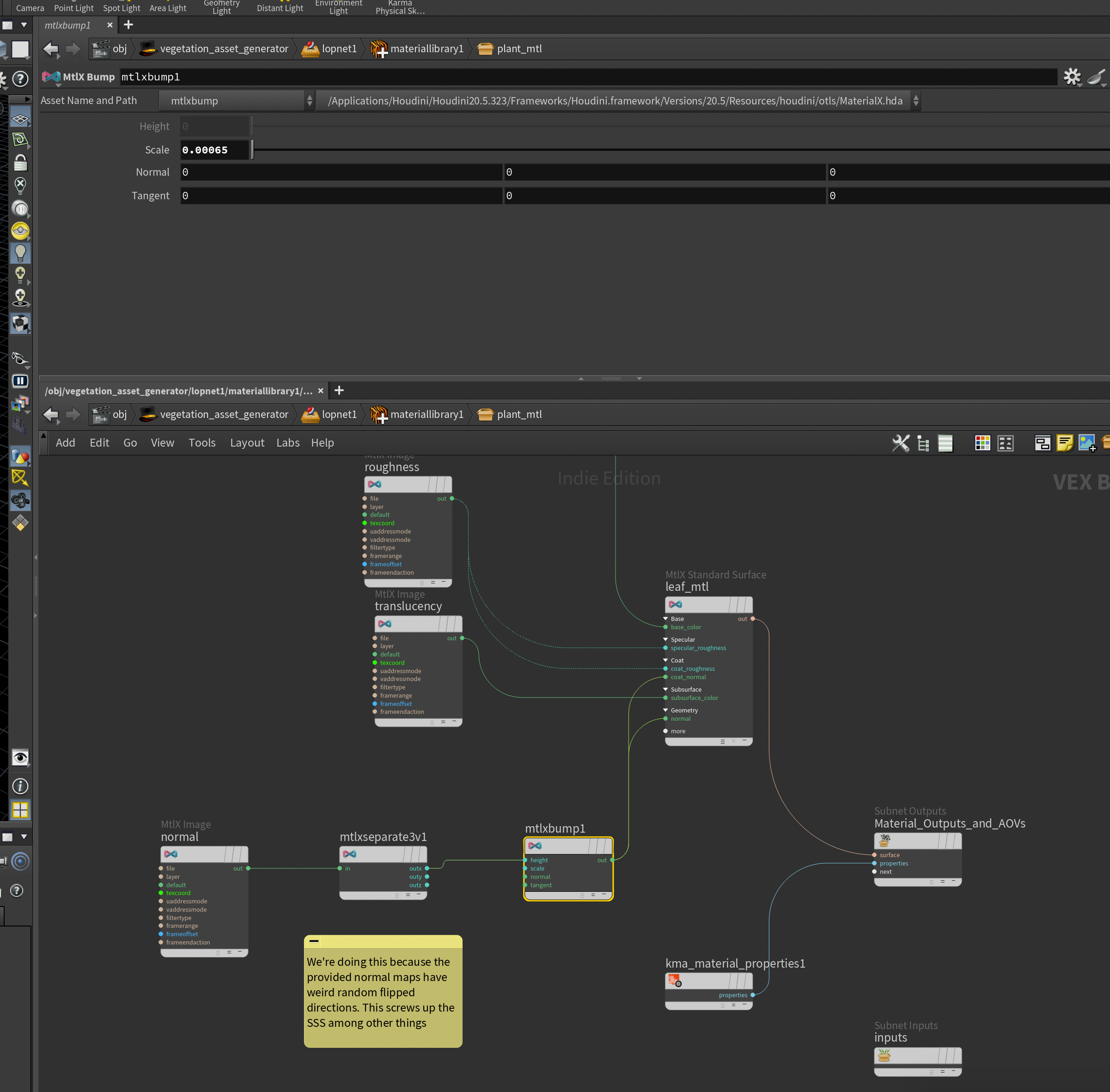
First, I've modified the normal map a bit by extracting one of the components of the normal map and using it as a bump map instead. The reason for this is unique to GScatter, as I found the normal maps to have some weird artifacts, unfortunately. There were a couple of areas in some of the textures that had flipped normal directions, which caused odd behavior in our SSS especially. So this was a quick and dirty fix to combat that. Also notice that I'm using a very low Bump scale of 0.00065 in the MtlX Bump node.
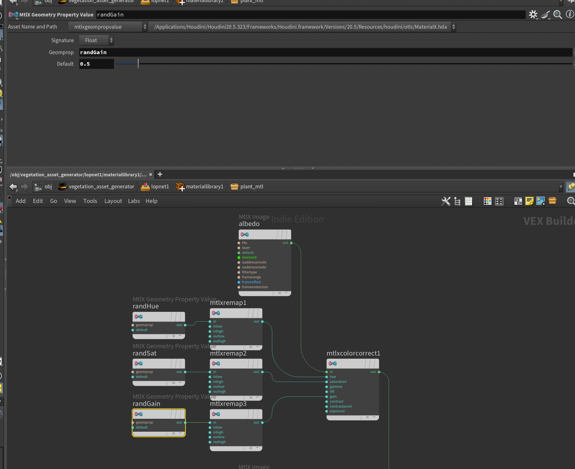
Secondly I created some MtlX Geometry Property nodes set to randHue , randSat, and randGain respectively and plugged those into a MtlX Color Correct that has the albedo as an input.
I did this so I can vary the hue, saturation, and gain between vegetation instances by adding the same attribute with a random value for each instance of vegetation. This helps create variation in our shading. All of them are set to 0.5 by default. After each MtlX Geometry Property Value I also plugged in a MtlX Remap remapping the Outlow and Outhigh to some sensible values (basically the min and max hue/saturation/gain that I want).
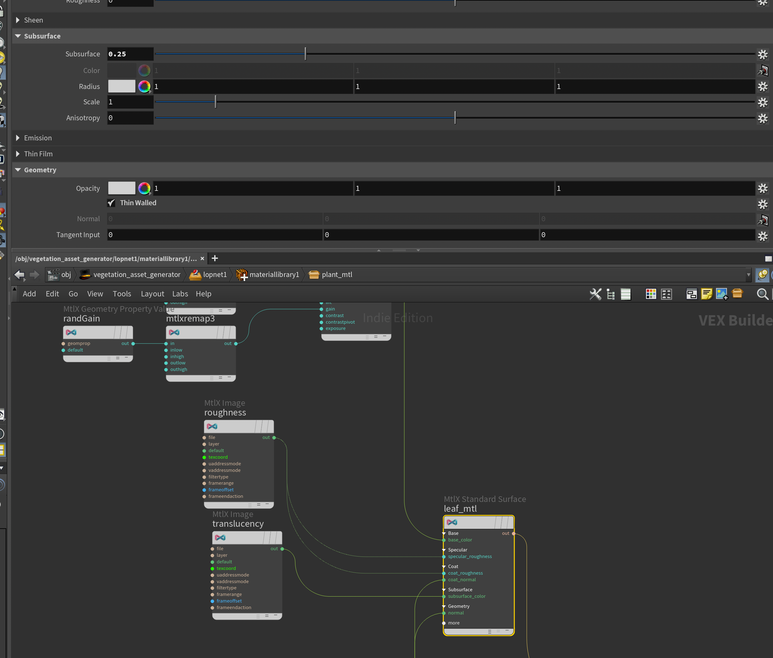
Finally, in order for the SSS to work (I use translucency as the SSS color) I set the Subsurface to 0.25 in the MtlX Standard Surface and turned on Thin Walled. This helps us add the nice translucency effect you get when light passes through leaves.
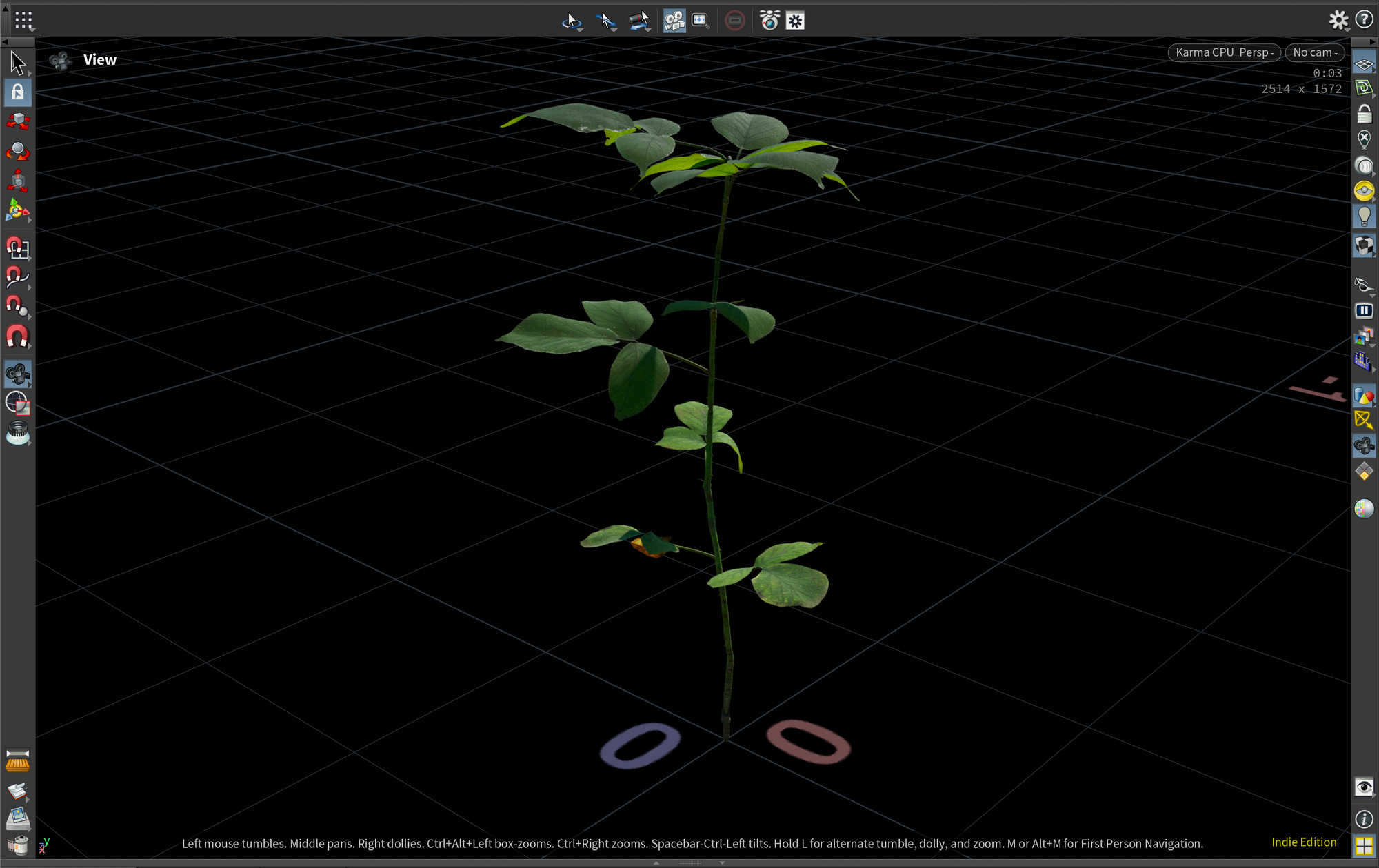
If you jump out of the material library, the Component Material node should automatically attach the output shader to the /ASSET primitive - resulting in a shader like you see below.
USD Export
With our USD setup ready we now need to write out our asset USDs to disk. Before we can fully do that we need to modify a few things in the Component Output node that comes after our Component Material node.
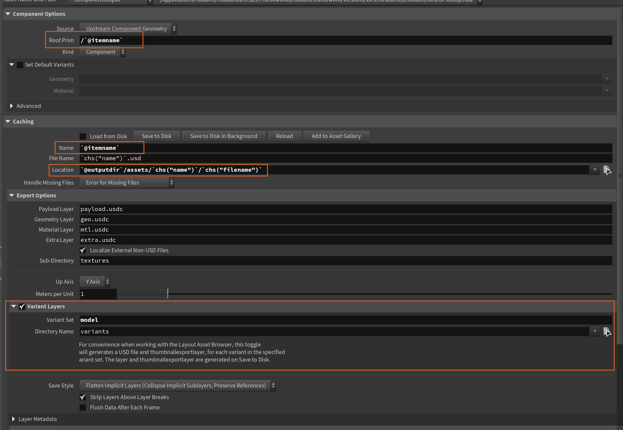
Root Prim needs to be set to the following, to make sure that the /ASSET prim gets renamed to the name of the current asset/workitem.
/`@itemname`Root Prim
We also need to do the same to the Name parameter under Caching, setting it to the following so the .usd files are appropriately named.
`@itemname`Caching -> Name
And the Location under Caching also need to be changed to the string below so that we get our outputs in the same root directory as our original assets (this can of course be changed if you want them somewhere else).
`@outputdir`/assets/`chs("name")`/`chs("filename")`Caching -> Location
And finally we need to enable Variant Layers and set the Variant Set to model. This ensures that the variants we've added to our asset get exported.
Back in TOPs, we simply need to add a ROP Fetch node to the end of our TOPs network that points to the ROP inside of our Component Output node as seen below. This will enable us to batch-export each vegetation asset through this LOP network and write it out to disk.
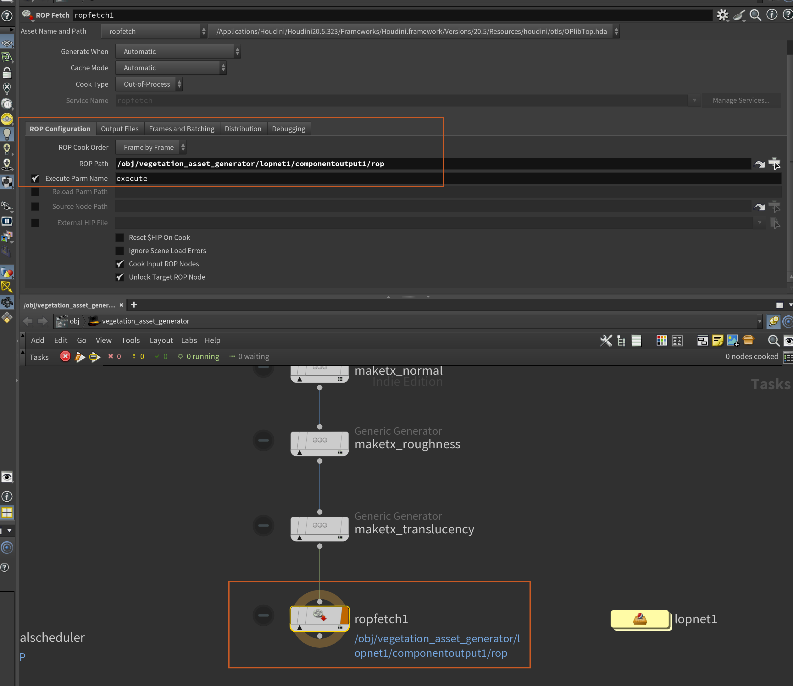
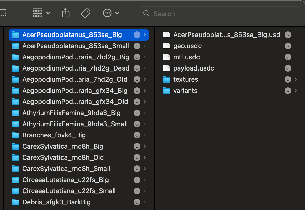
And that is the end of our setup. At this point in time, if you were to select the ROP Fetch node and press SHIFT+V you would execute the entire TOPs chain, exporting nicely organized USD files - complete with payloads, textures, and variant setups.
Conclusion
To be continued in Part 2...
This marks the end of the first part of this article. We now have a working USD Asset setup that we can run in a batch to process multiple vegetation assets and generate proxies, skeletons, and shaders in a clean and orderly output. In the next part, I will cover how to take these assets and add them to a layout, simulate an area of vegetation using Agents and Vellum, and finally render and composite the result you see below.
Final composited shot.
If you want to get notified when the next part comes out, please consider subscribing to my newsletter below!
Thank you all for reading, and see you for part 2!