Creating Procedural Drift Ice in Houdini using SOPs and Solaris
Lately, I've been chipping away on a larger personal project. In that process, I needed to create a bunch of drift ice to fill an arctic ocean. I thought some of the tools I used in this process might be handy for a few people out there, so I decided to type up a post describing some of the techniques in detail. I've tried to cover most of the techniques used in creating the scene below, from geometry generation in SOPs to shading and assembly in LOPs, using simple examples and GIFs. I hope you enjoy and learn something useful!
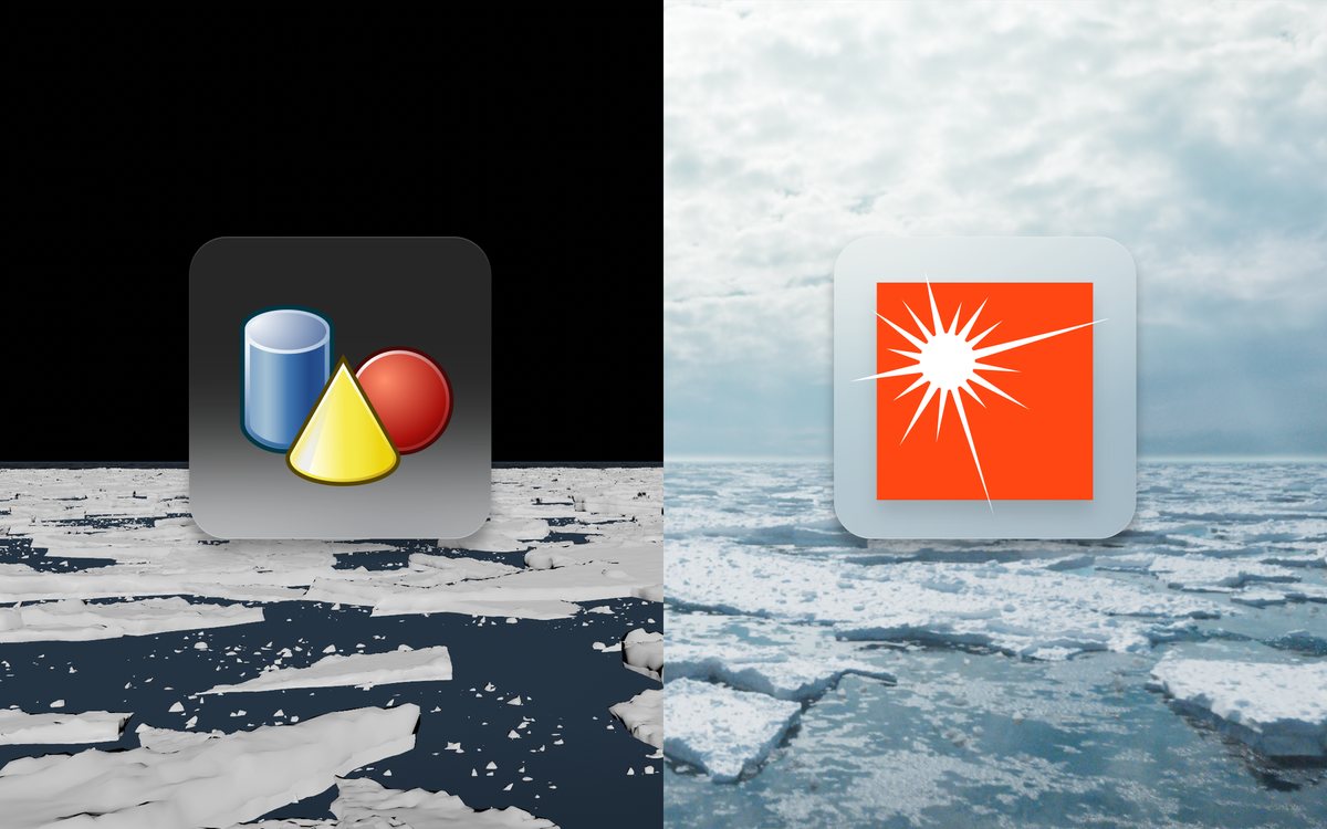
Final composited shot.
Geometry Generation
Creating the drift ice geometry in SOPs.
Generating Base Shapes with RBD Material Fracture
Finding a good base shape for procedural modeling is essential. In computer science, there's a good phrase - "Garbage in, garbage out". This is true for procedural modeling as well.
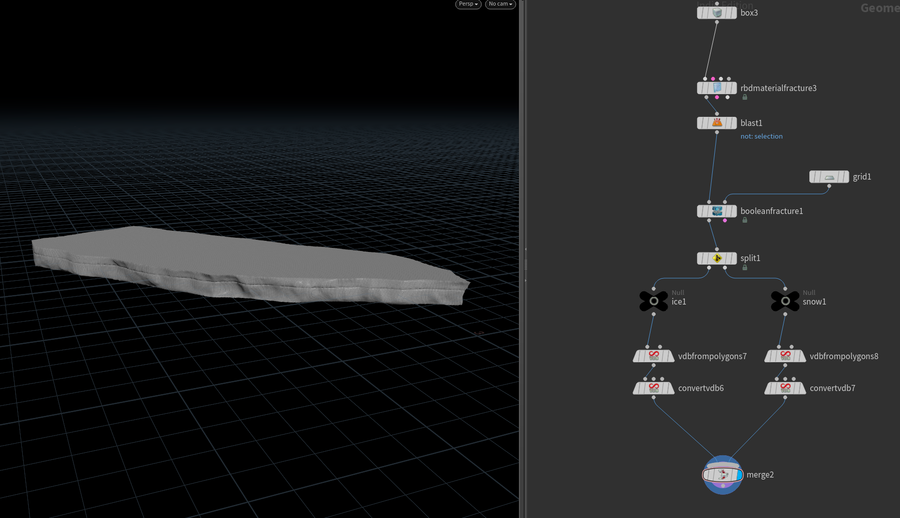
In this setup, I used the RBD Material Fracture node on a simple box geometry to create the base shapes. This node is commonly used for creating fractures for rigid body simulations but is just as useful for procedural modeling.
Fracturing geometry like this used to require some fairly complex setups (especially for some of the more advanced features of this node), but these days you can get a great result using only this node.
For this example I just used the concrete preset for the node, tweaked generation a bit, and turned on Interior Detail and Edge Detail in the Detail tab.
After this, to split the geometry into an ice and a snow section I used a Boolean Fracture node.
The Boolean Fracture is another RBD node. It takes two inputs - the geometry you want to fracture, and the "cutting surface". In this case, I just used a simple grid, but you can get creative with this and generate complex fractures. In hindsight, I could've also used a regular boolean node here, but the RBD Boolean Fracture generates a name attribute automatically which will be useful in the next step.
Adding Details using Attribute Noise
At this point I split the two parts (ice and snow) using a Split node, based on the name attribute, to detail them separately.
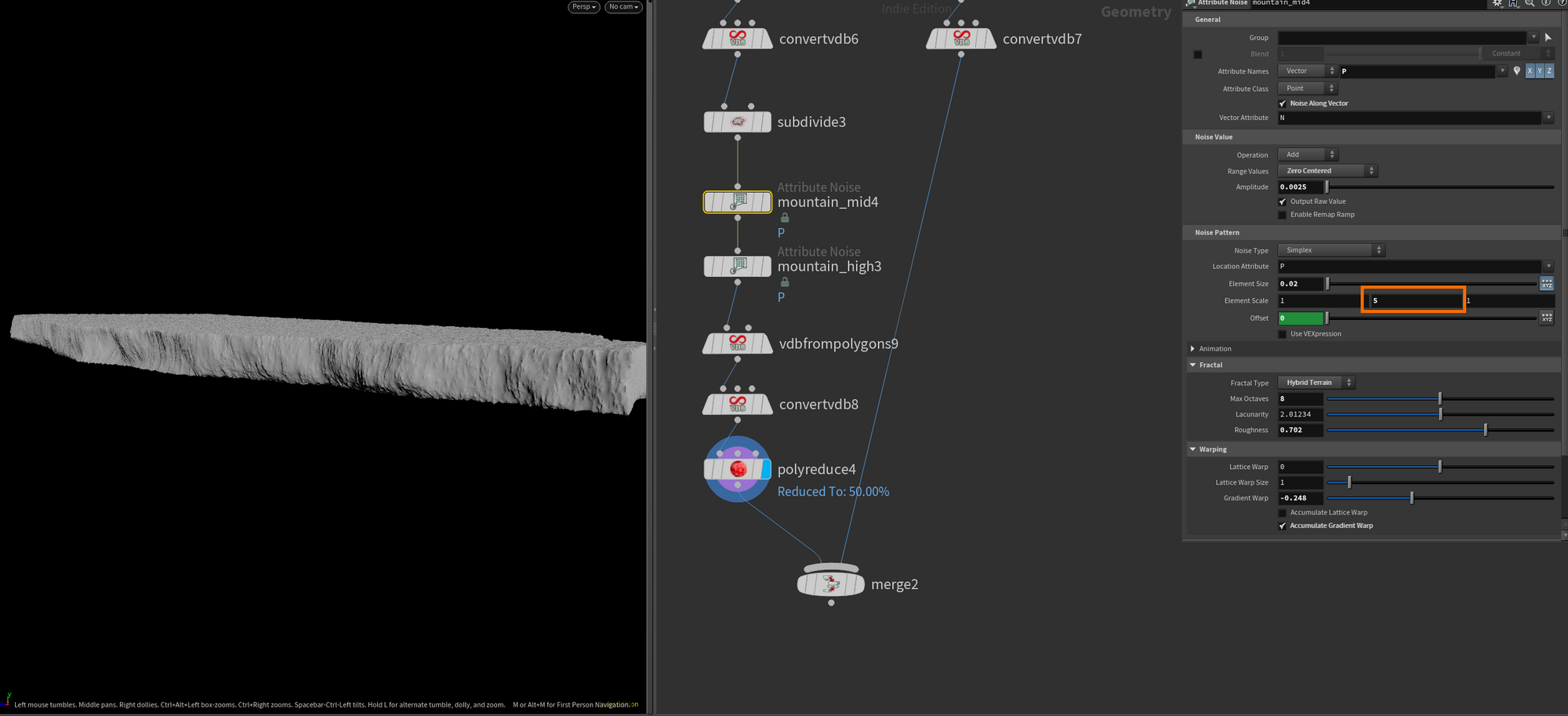
For both sides, I first converted the geometry to SDFs (surface VDBs) using a VDB From Polygons Node, and then back to polygons using a Convert VDB node. This is a cheap and effective way to get a more uniform polygon distribution. This will be very useful when adding procedural details such as noise.
From this point on I mostly just layered different noise types using Attribute Noise nodes. The only unique setting for the ice is that I set the y-component of the Element Scale to be relatively high compared to the surrounding components. This was done to get the streakiness you see in the screenshot below (which felt similar to the ice I was looking at as a reference).
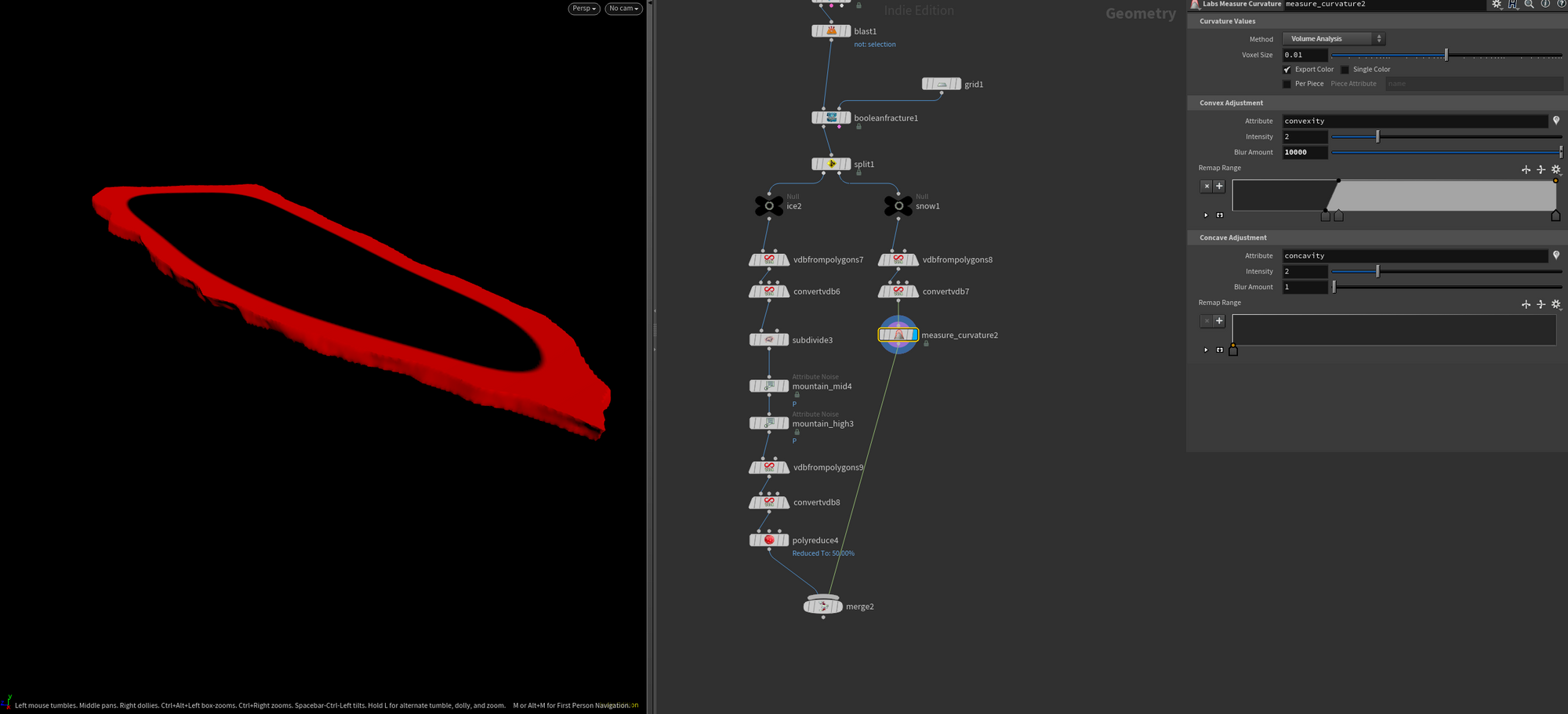
For the snow, I wanted to simulate an effect I noticed on some of my reference images of snow building up around the edges of the drift ice.
To achieve that I used a handy node from the SideFX Labs toolset (https://www.sidefx.com/products/sidefx-labs/) called Measure Curvature. This node allows you to generate various curvature-related attributes. Then, to only have the mask appear on top of the geometry I masked it based on @N.y in VEX like so:
float curvature = f@convexity * chramp("Remap", @N.y);

@mask = curvature;
The code essentially just allows me to multiply the convexity attribute generated in the Measure Curvature node with a ramp based on the Y component of the normals. Effectively this just means I'm making sure that the mask is only applied to points that have normals pointing up in Y.
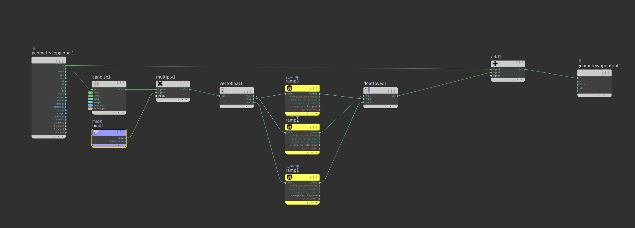
Finally, I added some noise based on this mask in a point VOP. The amplitude is set quite high since we want some pretty aggressive shaping.
After this step, I simply kept adding more noise layers, subdivided once, and did another roundtrip of generating a VDB from Polygons and converting it back to Polygons right after. This was simply to clean up a few artifacts in the mesh from some slightly extreme noise layers.
Adding additional details using scattering
An effective tool for adding complex details is scattering geometry on top of an existing mesh. In this case, I wanted to emulate a bit of "snow clumping" by scattering some simple snow clumps I created. I also ended up using these to add an extra layer of complexity to the final layout.
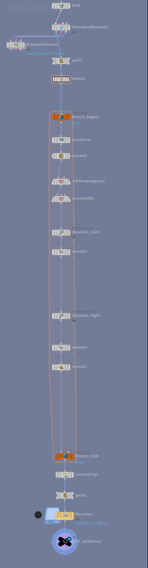
The network for these small snow clumps was very similar to how I generated the snow and ice above. I created a box, fractured it using RBD Material Fracture, and then ran them through a for each block where I added some noise to each piece and moved them to the origin. Finally, I cached them out so I wouldn't have to keep recomputing these. The most important part is assigning a name attribute to each piece. I've done this here using the Connectivity node.
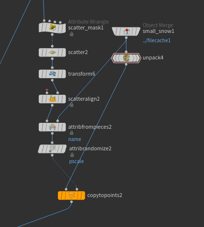
After this, I piped the result of this graph into a Copy to Points node and scattered them on the drift ice based on points generated by a Scatter node with density mapped to a mask.
The mask was generated like so in VEX, similar to the previous snippet I shared. All it does is make sure we get most of our points on the top of the mesh where the normals point in positive Y.
f@mask = chramp("Remap", @N.y);I don't want to go into too much detail on scattering in this guide, but I used a combination of Attributes from Pieces and Scatter Align to orient, set pscale, and randomize which piece got assigned to which point.
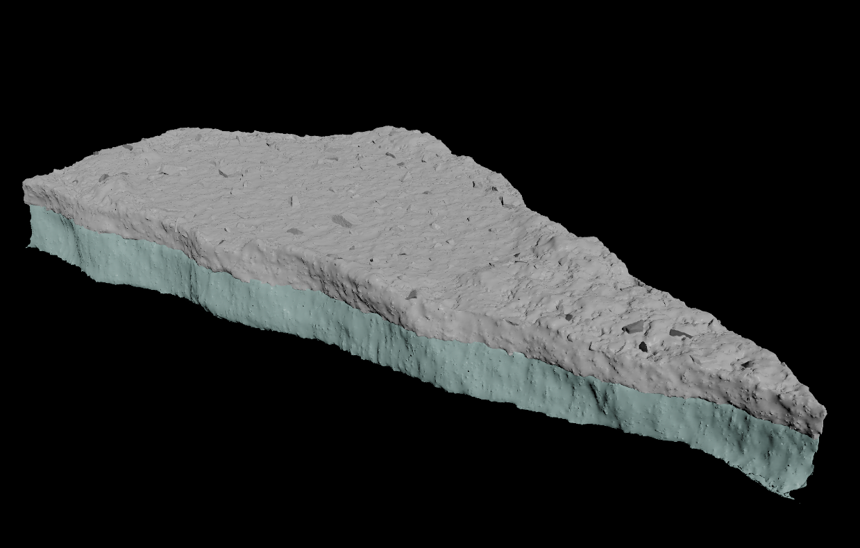
Now, after merging this scatter setup with our ice and snow meshes we end up with something like the model below!
Setting up For-Each loop for fast variants
The last step before we move on to prepping the model for USD/Solaris is setting up a For-Each loop that allows us to generate multiple variations of the model using the same node tree.
Setting it up requires you to add a For-Each Named Primitive block after the initial RBD Material Fracture. And essentially just plotting all the detail generation in between the begin and end-node of the For-Each block.
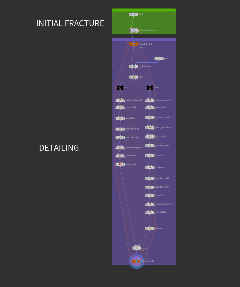
Through this, you'll then be able to generate a finished model for each fractured piece. You may even be able to throw areas of this graph into a Compile-Block for multithreading.
If you want to center each model you can add a transform node at the beginning of the For-Each Block setting the translate x, y, and z to the negative centroid. This effectively places the center of the mesh at the origin.
Translate X: -centroid(0, D_X)
Translate Y: -centroid(0, D_Y)
Translate Z: -centroid(0, D_Z)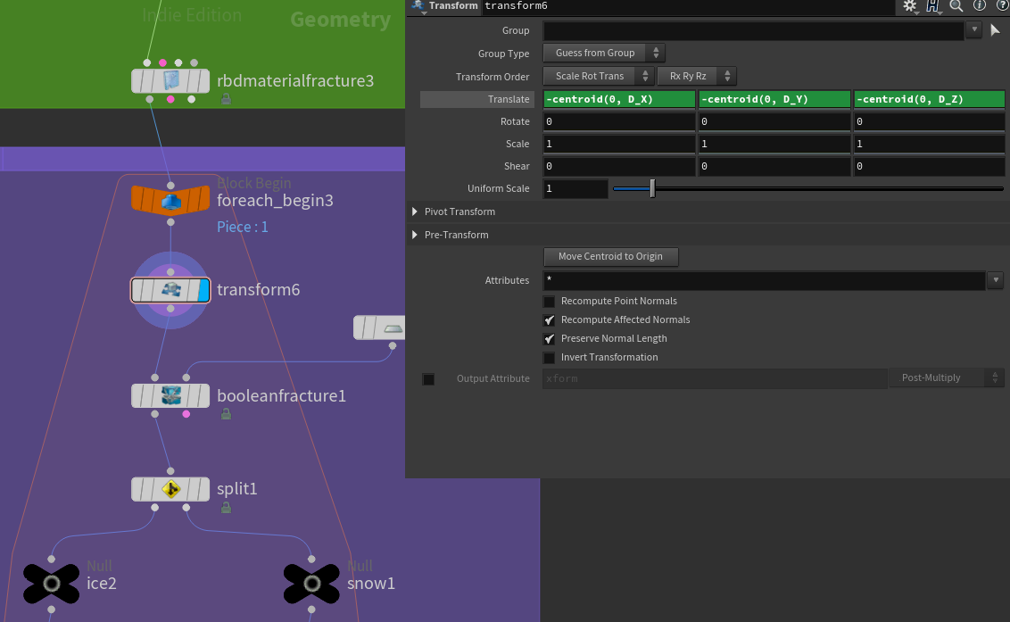
Another great thing to do is vary the noise offset per piece. You do this by using the iteration detail attribute generated by the Meta Import Node. To add the Meta Import node click this button in the For-Each Begin node:
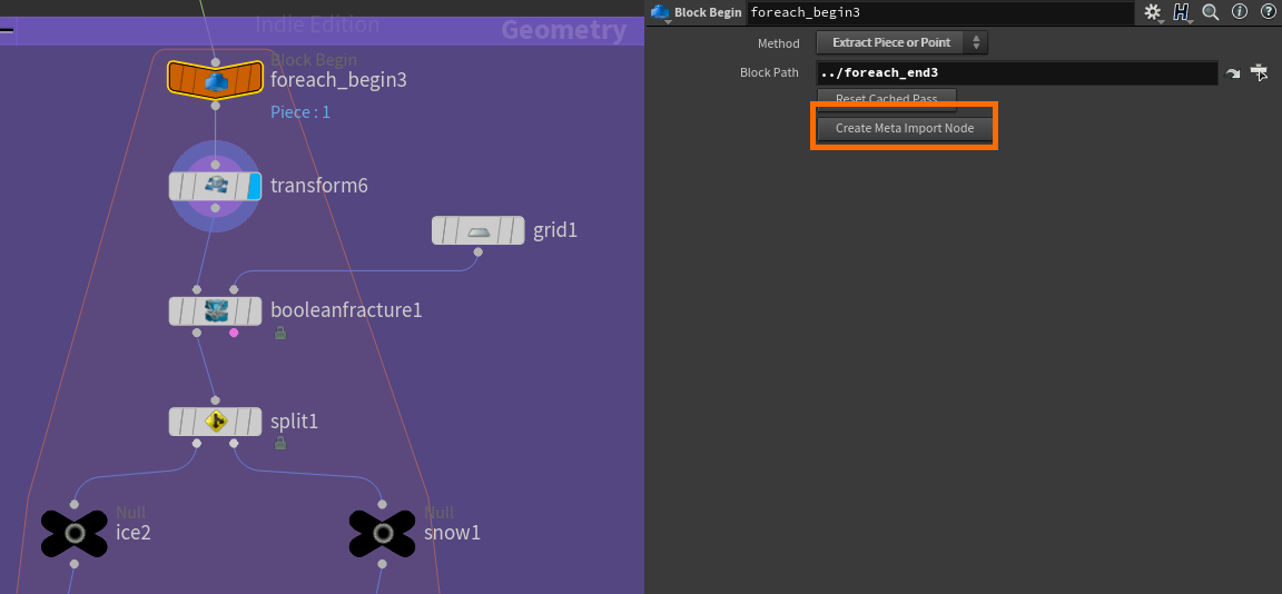
This will create a new node in your network that you can reference to access the current iteration number among other things. For example, you can use it in a Noise Pattern Offset like so:
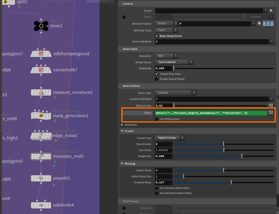
detail("../foreach_begin1_metadata1/", "iteration", 0)Quick Tip: Cubic UV Projection in VEX
Before we fully leave SOPs I wanted to share a script I used to generate UVs for these models. I wanted to do procedural UV generation so I could create as many variations of my models without having to worry about creating manual UVs.
UVs can be quite tricky to generate procedurally, but I found a great VEX snippet while working on this project courtesy of Konstantin Magnus. It generates a Cubic UV Projection which worked quite well in my case. He wrote a post about it here: https://procegen.konstantinmagnus.de/cubic-uv-projection-in-vex
Prepping geometry for Solaris
Prepping and exporting geometry through LOPs.
Setting up proper Name Attributes from SOPs and creating proxies
I know I promised we were done with SOPs, but we need to do one last thing that's heavily related to USD and LOPs/Solaris.
If you've ever had the pleasure of importing content from Maya into Houdini you'll know that each piece of geometry has its path in the Outliner/Scenegraph stored as a string value in the path attribute. For example, if you create a "box_geo" object in a group called "box_grp" in Maya and export it to Houdini it'll feature a path attribute with a value of "/box_grp/box_geo".
Since USD (and by extension Solaris) also works with a hierarchy-based scene description it has a similar system. When importing geometry from SOPs to LOPs, the values stored in the name attribute can be used to tell USD where in the scenegraph it should place the geometry.
So, for each geometry in the For-Each loop, I added two Name nodes. One for the full-resolution render geometry, and one for the proxy geometry (I'll discuss this in the next section - fear not!). I used the same feature of using the iteration detail attribute from the For-Each metadata node to make sure that each iteration had a unique identifier.
The render geometry got a name attribute like so: iceSlab_grp/iceSlab_#/render/ice_geo
The proxy geometry got a name attribute like so: iceSlab_grp/iceSlab_#/proxy/ice_geo
Lastly, the render geometry and proxy geometry are the same geometry except the proxy version has had an aggressive polyreduce applied to lower polycount.
Preface: USD Purposes
So what are we going to use this low-resolution geometry for? The proxy geometry will function as a viewport preview of our geometry when doing layout and other tasks in the viewport. This way we can avoid loading the heavy geometry until we have to do our final rendering - significantly speeding up our workflow.
This approach is used a lot in production and USD even has a built-in feature for this type of workflow: USD Purposes.
To be a bit pedantic USD Purposes is a built-in attribute available on primitives using the UsdGeomImageable schema. But all you need to know is that it's a feature available on all common types of geometry you'll work with in USD/Solaris.
It's a little attribute that has 4 different settings. It can technically be used however a DCC wants, as it's just a hint from USD on how your DCC should interpret the primitive. But this is generally how it works:
- default = no special purpose, primitive is visible in all modes
- render = primitive is only visible in final render
- proxy = primitive is only visible in viewport
- guide = special purpose for applications who only wants to display guides (I have yet to use this purpose type personally)
They're the building blocks of USD.
Loading Geometry from SOPs into LOPs and setting up Purposes and Variants
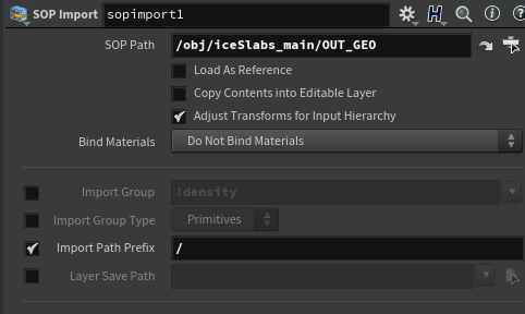
First things first, in order to load our geometry into LOPs (Solaris) we open up our /stage context and add a SOP Import node. This node is very straightforward and simply allows us to specify a SOP path that we can import straight into LOPs. In order to take advantage of our name attribute fully I also recommend you turn on "Import Path Prefix" and set it to /.
Now that we've done this we run into a problem. We would like to be able to only use one drift ice piece at a time, but right now they're all visible at the same time. USD has a fantastic feature to solve this called Variants. They'll become even more important when we get to the layout stage.
Variants allow us to have several different variations of an object. We could have versions with different shaders, or versions with completely different geometry. In our case though we just want to switch between each variation of our drift ice.
We could do this manually, but because we have so many I'd like to use a For-Each loop to generate them.
Because we are modifying existing primitives we need to plug in the scenegraph into the first input of the For-Each end node as well as the For-Each begin node.
Now, to create variants we need to create an Add Variant node (choose the Add Variant to New Primitive from the tab menu). We wire the For-Each begin node into the first input of the Add Variant node and add an Isolate node with a prim pattern set to `@ITERATIONVALUE` into the second input like in the screenshot below.
`@ITERATIONVALUE` points to the path of the primitive in the current iteration of the loop.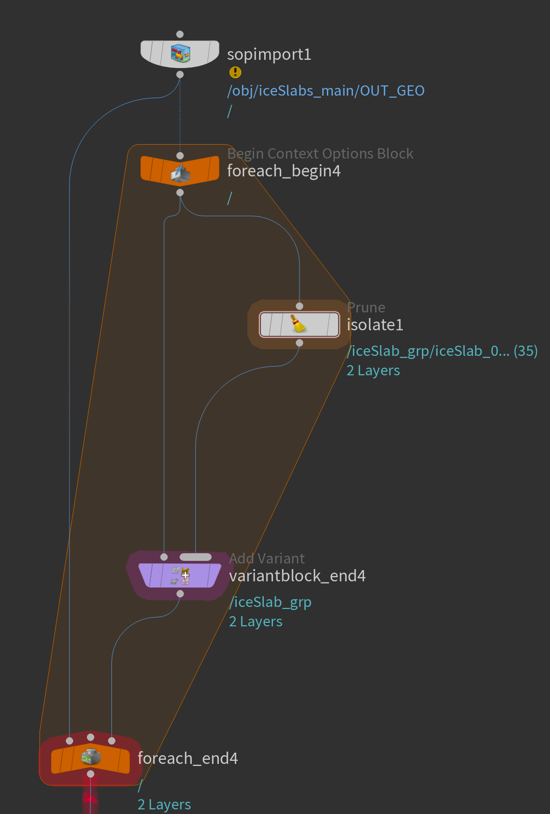
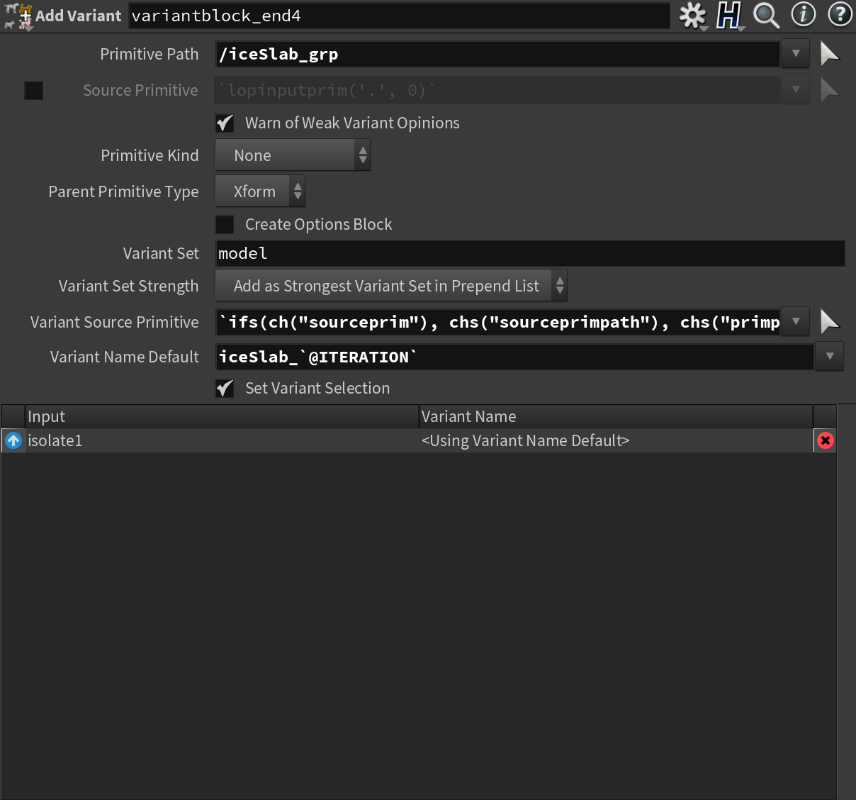
In the Add Variant node you simply need to set the Primitive Path to the top group (since this is where we want to allow the user to change variant from) and set the Variant Name Default to iceSlab_`@ITERATION` . This will be the name of our variant.
With this done we would like to set the geometry we put into our /render/ paths earlier to only activate at rendertime, and the geometry in our /proxy/ paths to only activate when we're looking in the viewport.
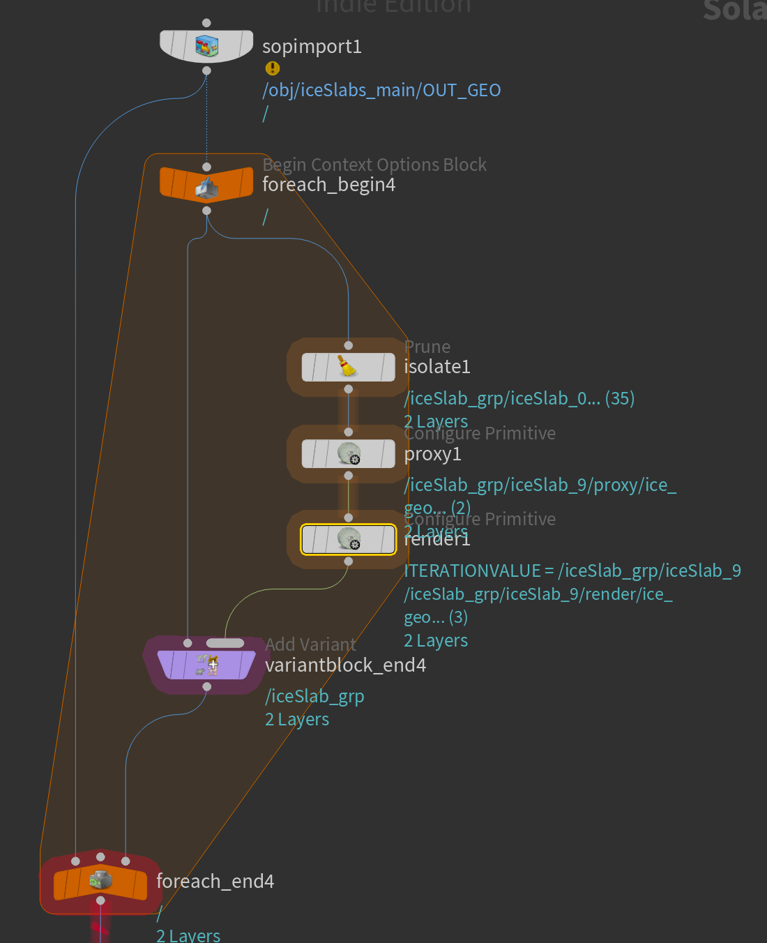
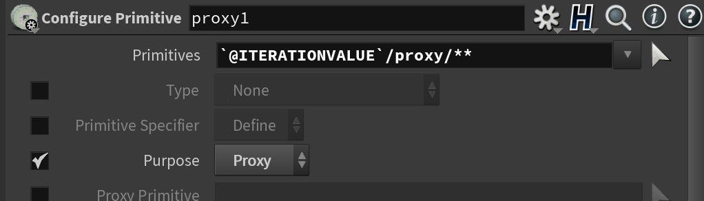
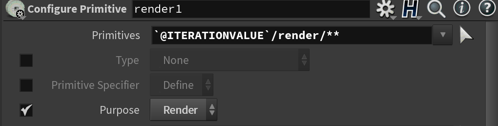
Since we already have a For-Each loop we can simply add a Configure Primitive under our Isolate node and target the proxy and render geometry respectively. See the screenshots below on how it is set up.
I use the Configure Primitive node daily, it is incredibly useful. And for our use-case, it has options to set Purpose built-in, so we don't need to write any manual code.
With this done we simply need to write out the result of our For-Each loop to a .usd file using a USD ROP and we're ready for shading, layout, and rendering!
You can test your new variants using a Set Variant node targeting the primitive you configured the variants on.
Layout & Rendering with Karma
Getting to the final pixels!
Setting up materials in Karma
This next section will be a little shorter as the render-setup and shading is fairly simple for this scene.
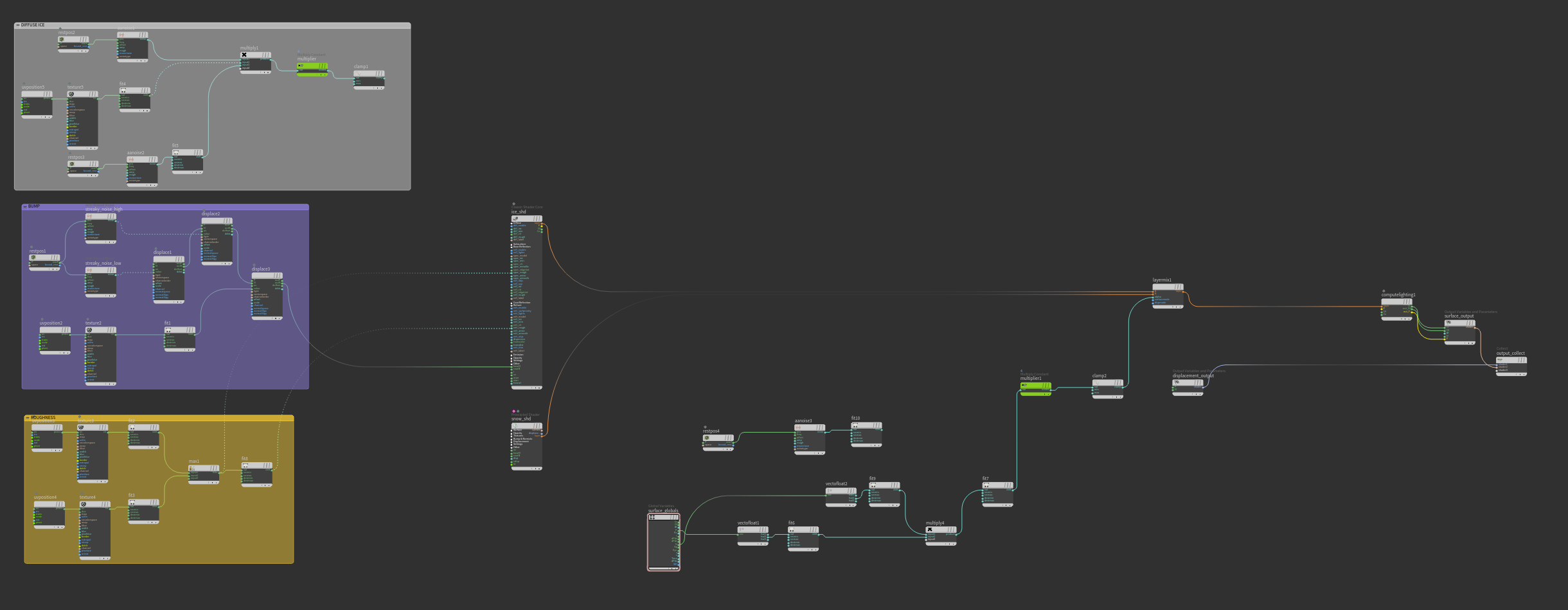
The model .usd file was loaded using an Asset Reference node (could also have used a regular Reference node) and shaders were added using a Material Library.
I'll cover my overall material workflow at a later date, but the snow and ice are essentially just created using a combination of Subsurface and Refraction with a slight blue tint in the ice refraction. I used a Classic Shader Core shader to build my material. Different layers of noise were added to create variation in the overall surface.
Final turntable
Layout in Karma
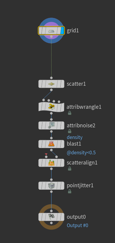
The layout process for this shot was also very simple. I animated a simple camera move, created an ocean using a grid from a SOP Create with some noise in the displacement and a fully reflective and refractive shader.
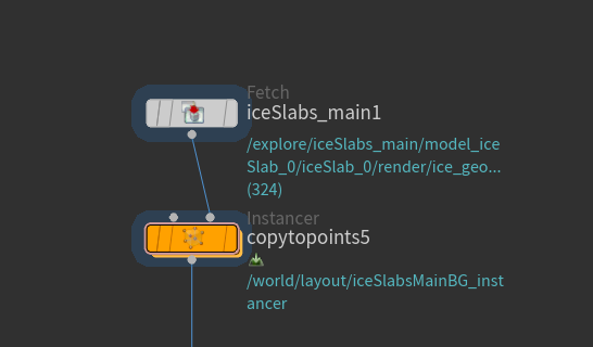
I then scattered the drift ice using a Copy to Points node (which is just an Instancer node with some presets). If you dive inside the Copy to Points node there is a SOP context where I added a large grid and scattered some points on it. Essentially the instancer will scatter primitives on the resulting points of the SOP context inside.
Lighting in Karma
Lighting for this scene was incredibly simple as it just consisted of an HDRI. Normally I would paint out the sun in the HDRI and add my own directional light, but in this case, the HDRI worked perfectly as is.
I got the HDRI in this scene from https://polyhaven.com.
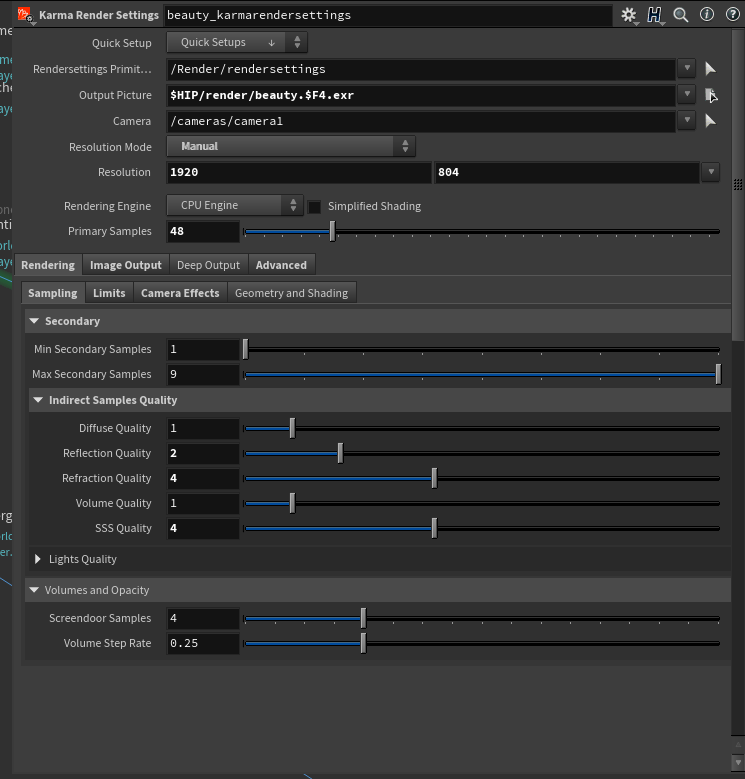
For render settings, I just boosted the Reflection, Refraction, and SS Quality a bit and used a Primary Samples count of about 48. The render was around 30 minutes per frame on an M2 Ultra Mac Studio using the CPU Engine.
Here is the final shot:
Final composited shot.
Bonus: Creating custom AOVs based on primvars in Karma
Before I end this article I quickly wanted to cover how to create AOVs in Karma based on Primvars. This can be useful for a lot of cases when you need to have a little more flexibility in compositing.
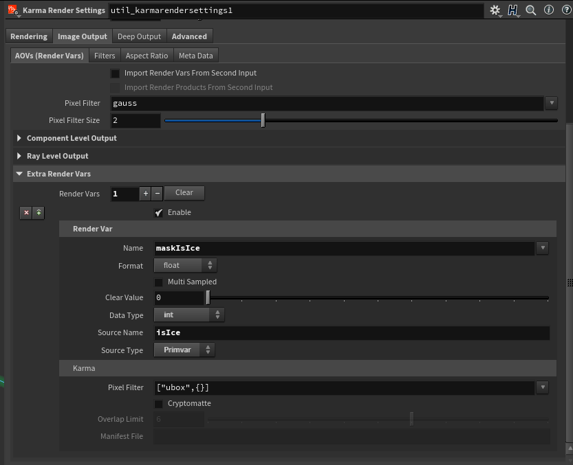
You can do this very easily in the Karma Render Settings by scrolling to the bottom of the Image Output tab and opening the Extra Render Vars panel.
Here you can specify a name for the AOV in the "Name" parameter as well as the Data Type and Source Name of your Primvar. Also, remember to set the Source Type to Primvar.
If you aren't familiar with primvars I recommend reading about them in the excellent USD Survival Guide by Luca Scheller: https://lucascheller.github.io/VFX-UsdSurvivalGuide/core/elements/property.html#attributePrimvars
Essentially it's a special attribute namespace that ensures an attribute is exported to rendering. It is useful for adding attributes that need to be accessed by shaders and AOVs.
Conclusion
Just wanted to say thank you if you made it this far! I'm aiming to write more of these types of articles in the future. If there's anything you'd like to see covered don't hesitate to type a comment below.
I would also love to hear if you were able to use any of these techniques in your own projects.
If you want to get notified when I post more articles feel free to subscribe below!