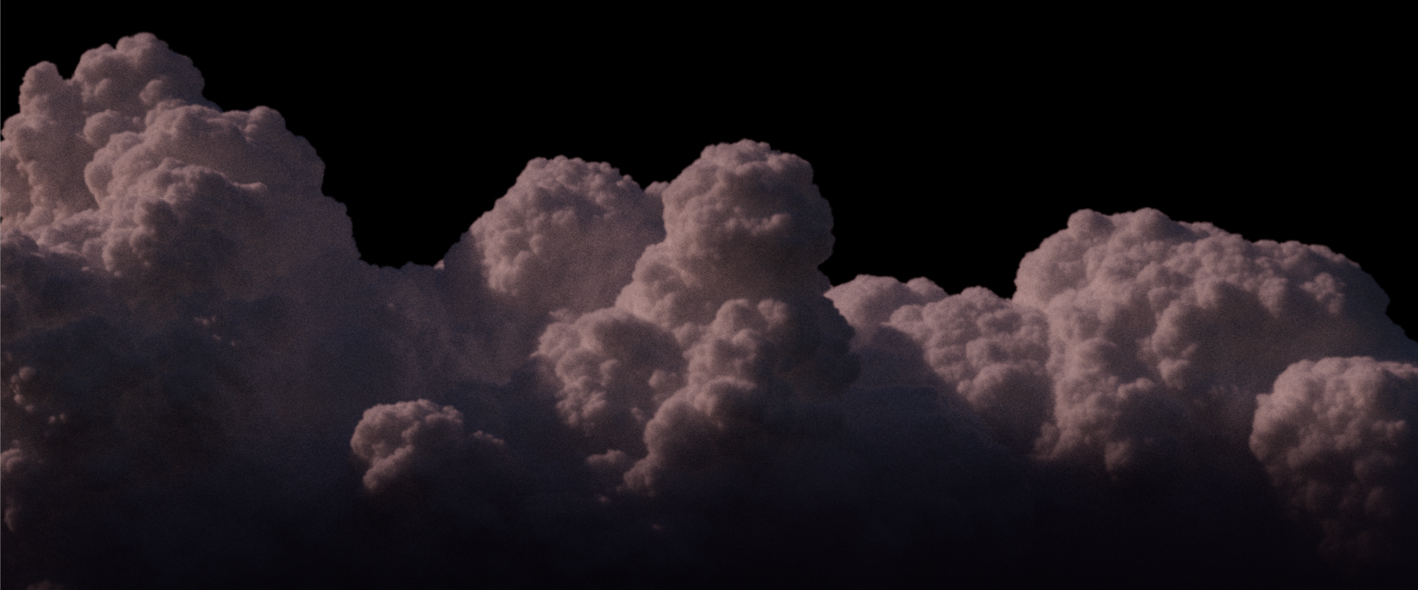
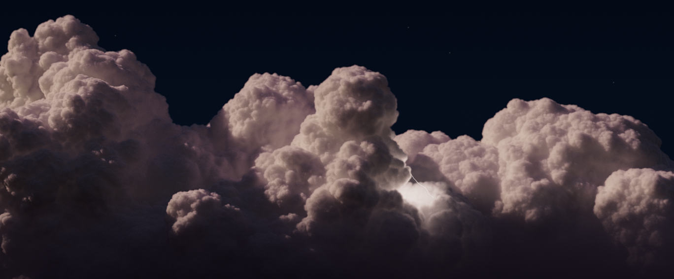
Thunder Clouds in Houdini 20
Learn how to make imposing thunder clouds using Houdini 20 and Karma.
In Houdini 20 SideFX introduced some very efficient tools for creating clouds and cloudscapes. In this tutorial, I'll use those tools to create an imposing cloud formation and extend the toolset by adding a SOP Solver for custom advection (to add subtle movements to the cloud), and generating lightning strikes within the clouds.
I'll cover the entire process, from modeling, simulation, rendering, and final compositing. I hope you enjoy it, let's begin!
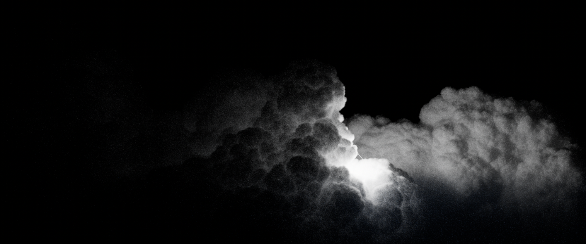
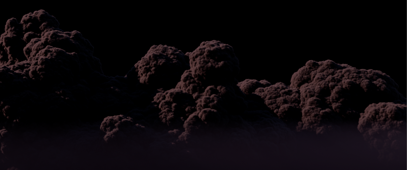
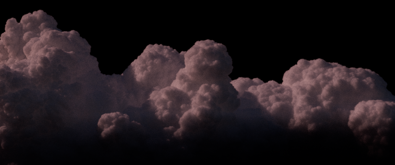
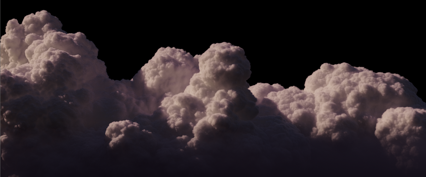
Final composited shot
Cloud Modelling
Exploring the new cloud tools in Houdini 20
Cloud Shape Generate
As I mentioned in my previous tutorial Creating Procedural Drift Ice in Houdini using SOPs and Solaris one of the keys to generating nice procedural models is to have a good base. The same goes for creating clouds.
Luckily SideFX has provided us with a new node in Houdini 20 called Cloud Shape Generate. This node generates particles with pscale (used to set the scale of particles) in formations that are meant to look like clouds. This is not the only way to generate a base shape for clouds, but I find it to be the most natural-looking.
The node can be a little daunting at first as it has a lot of parameters, but I'll cover the ones that I used the most in this project. Hopefully, this will help you get a good starting point for your clouds.
Shape
The shape section contains several general parameters for the cloud shape. Here are some of the key ones you should adjust first.
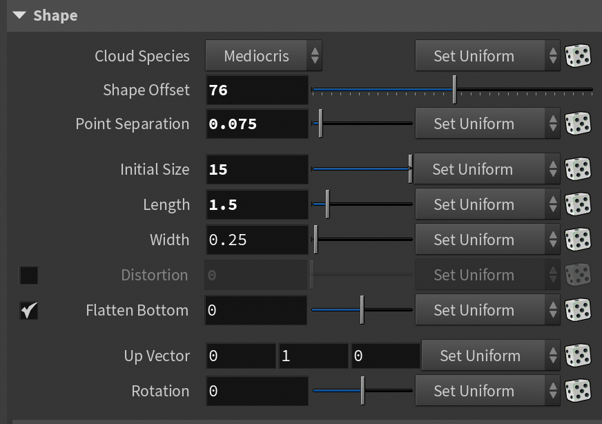
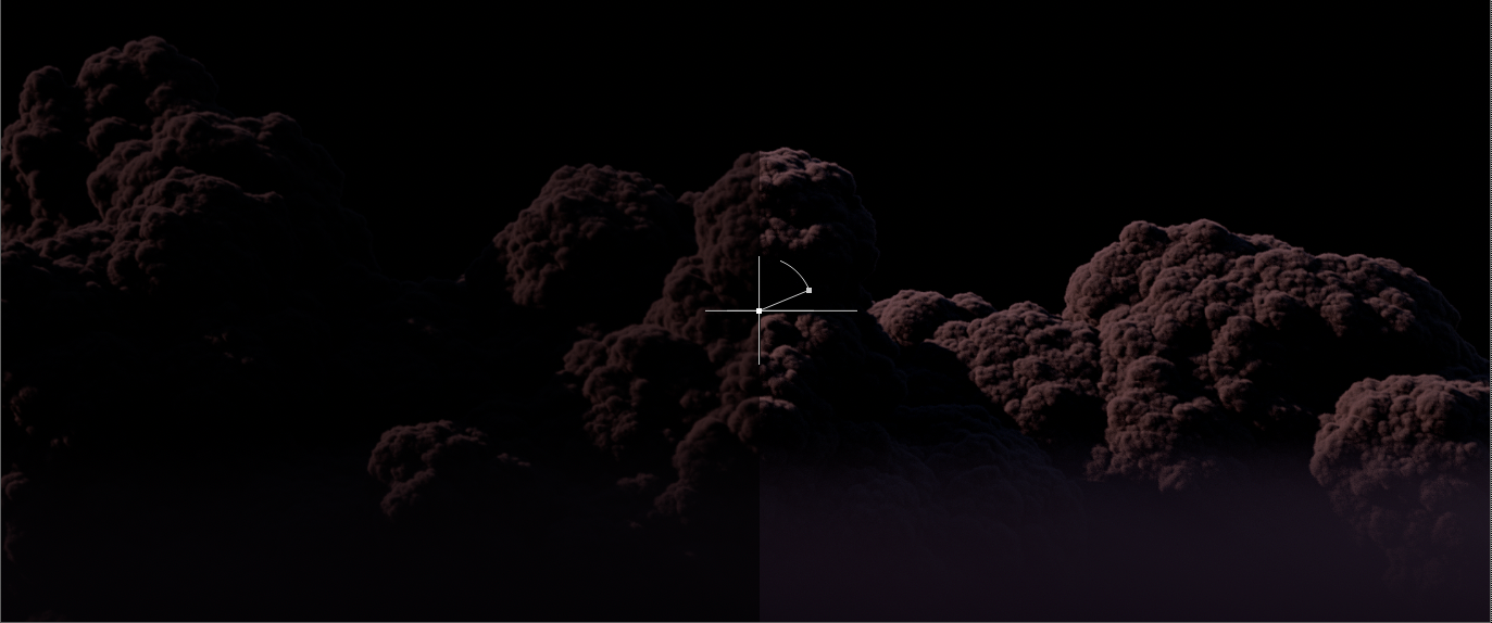
Cloud Species - At the time of writing there are 3 different cloud species in this list. Mediocris, Humilis, and Congestus. Humilis is a very low, almost flat cloud type. Congestus is the opposite, a very vertical cloud similar to what you'd see in a thunderstorm. Mediocris is a nice in-between which allows the best of both worlds. You get the towering effect but also a bit of width at the bottom. I used Mediocris for 80% of the shot in this tutorial, the remaining being Congestus.
Shape Offset - Effectively allows you to randomize the shape. Can be useful when trying to generate several clouds using the same setup.
Initial Size / Length / Width - Basic size settings, I recommend dialing these in first.
Secondary Shapes
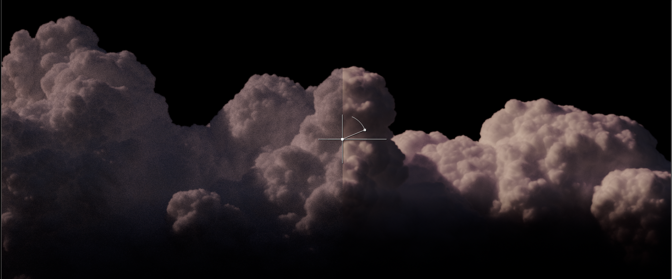
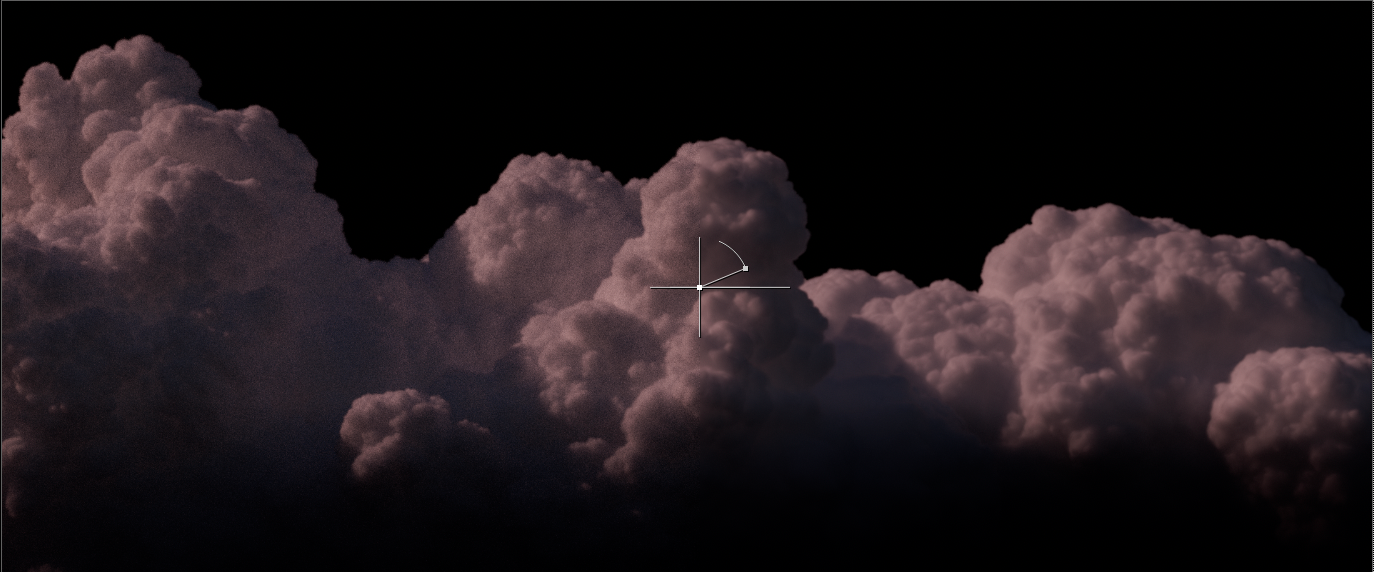
This section of the Cloud Shape Generate node offers what I consider to be some of the most important parameters for getting a natural-looking cloud. It allows you to "grow" your cloud vertically, creating beautiful silhouettes. See the examples below on how to use it:
Iterations - How many times secondary particles are generated. Think of this as the growth steps.
Displacement - This option controls how far along the up vector (usually the world Y-axis) the displacement goes. Think of this as the amount of vertical growth.
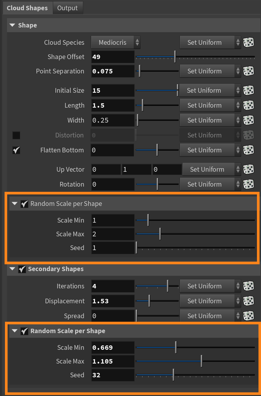
Random Scale per Shape (1 & 2)
If you look at the Cloud Shape Generate node you'll notice that there are two Random Scale per Shape sections. It's not explained very clearly in the node, but it allows you to add two separate layers of random scale based on noise. I advise you to enable both of them as it helps create a lot of nice variation. There aren't any magic values here, but I've included an example from one of my clouds here.
Go ahead and experiment with the settings in this node and see what you can come up with! You can even merge several different Cloud Shape Generate nodes to form even bigger clouds.
Cloud Shape Replicate
Cloud Shape Replicate is another useful node. It takes an input point cloud (usually a Cloud Shape Generate node) and scatters points on top of the existing cloud shapes.
The primary thing I've changed here is turning on Scale Along Direction and Align Along Direction (I've set it to the Y-Axis as you can see in the Direction parameter). This makes it so the additional spheres/points are formed more densely around the top of the cloud. I think this mimics real clouds pretty well - having the smaller scale detail concentrated towards the top - and hinting that there's an upward expansion.
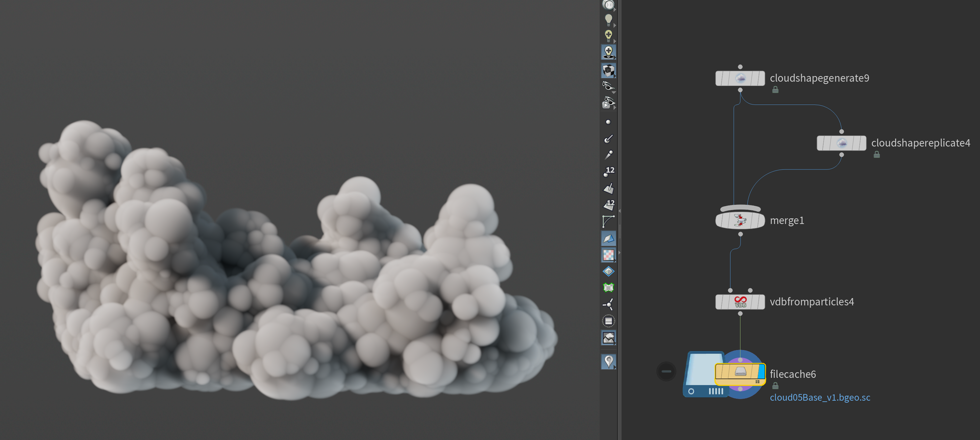
I then merge the result of this node with the previous Cloud Shape Generate to form the final base shape.
Volume Generation
With our base shape ready, it's time to move into volumes and start generating our fine details. First, we'll need to convert our base shape into a VDB Density field (also known as a Fog VDB).
Doing this is quite straightforward too, but it surprisingly doesn't require any custom cloud modeling nodes. We simply do it using a VDB From Particles node.
This node takes an input point cloud and turns them into a VDB (SDF or Fog VDB) using the pscale as a guide for scale. This is perfect for the output of our Cloud Shape nodes since in essence, all they do is output a point cloud with pscale.
Usually, the only thing you need to tweak in this node is the Voxel Size. In this example, I'm using a value of 0.07 but this will depend heavily on the scale of your cloud. I'm usually aiming for around 10 million voxels to make sure I have enough resolution for the finer details.
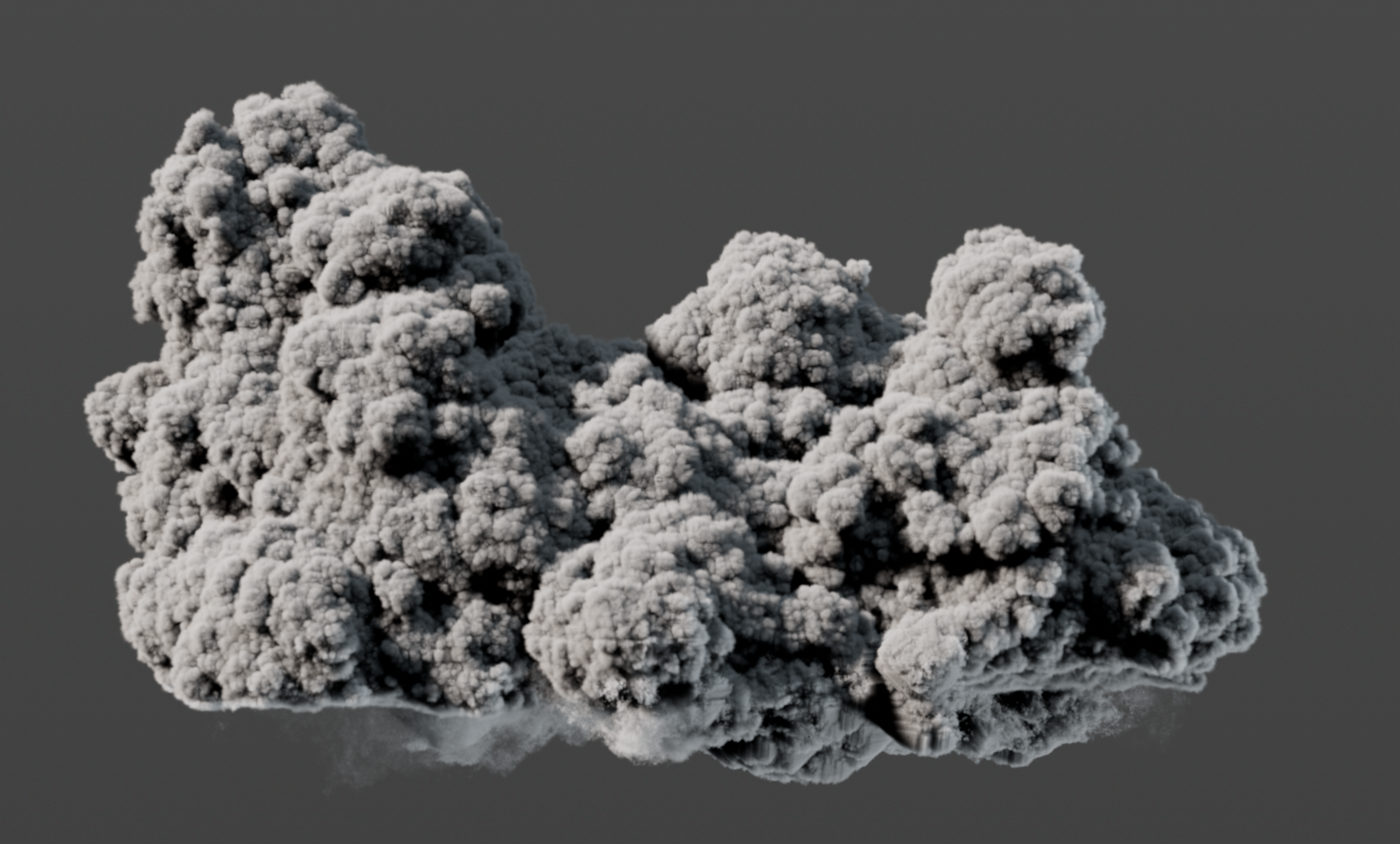
Cloud Billowy Noise
Great! We now have a volume. But it doesn't quite look like a cloud does it? This is where our volume noise generators come in.
In Houdini 20 SideFX a new noise generation node specifically made for clouds was introduced (although it could certainly be used for other things too).
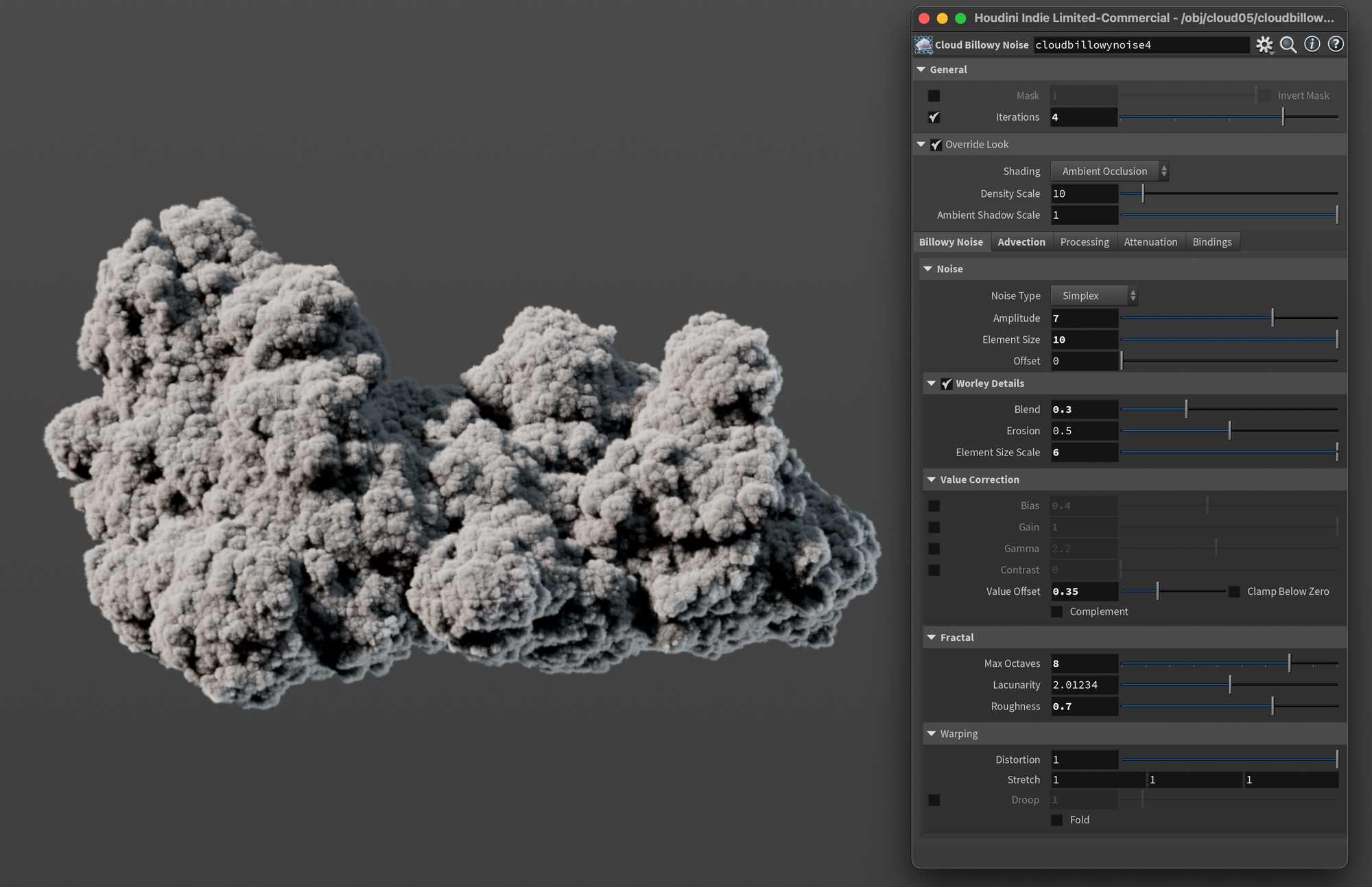
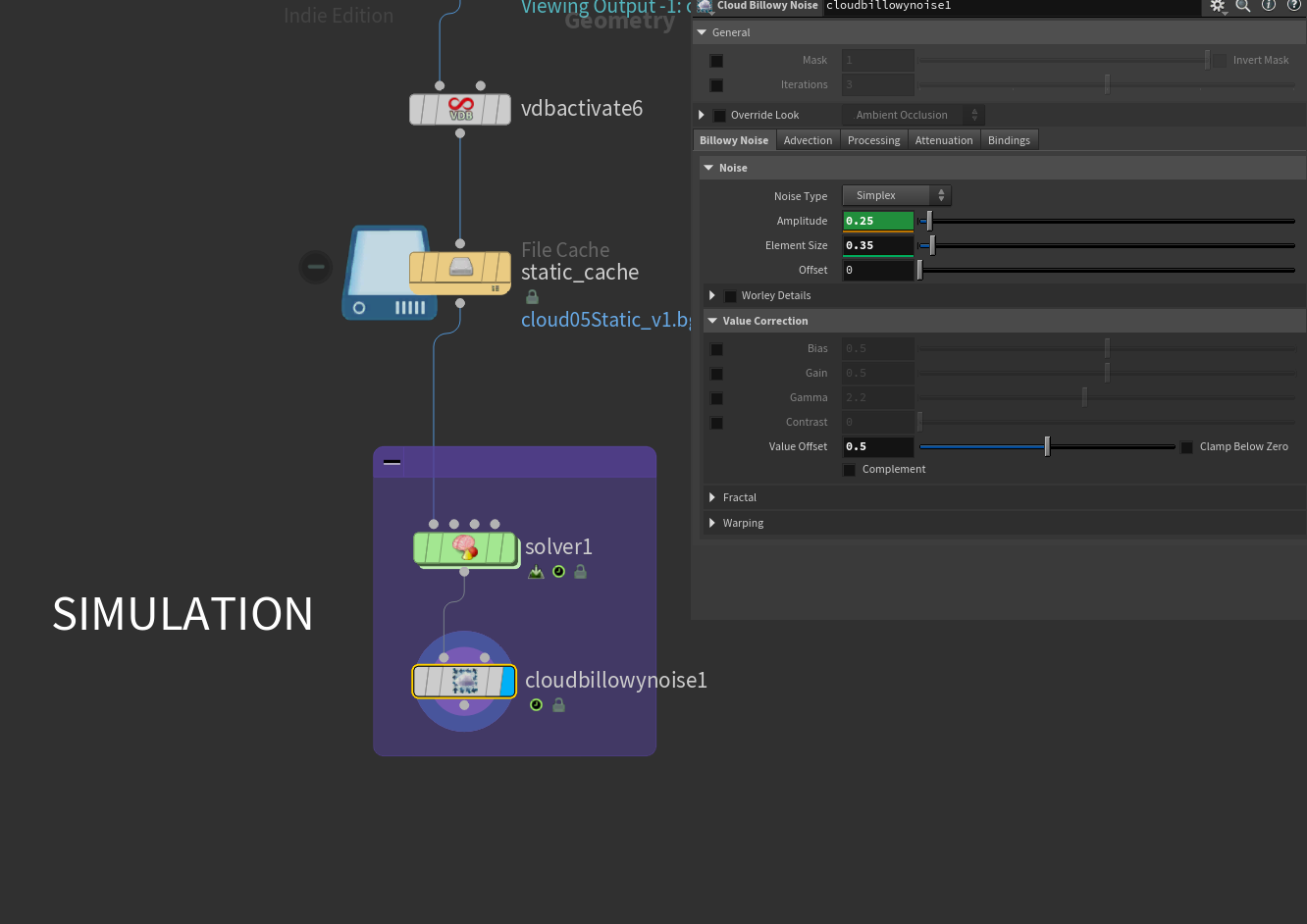
Like the previous nodes the parameters in this node are also very dependent on your input. But I'll share some of the parameters I like to dial in below. Above you can see the settings I used for this particular cloud (click the image to enlarge).
Iterations - This is the amount of displacement iterations of the noise. SideFX recommends to increase this number, and I have to agree. I found a value of 4 to work well across most of my tests.
Noise - Amplitude and Element Size - These two parameters are likely where you'll spend most of your time. They determine the look heavily. Element Size is the size of the noise, and Amplitude is the strength/intensity.
Worley Details - This section is disabled by default, but I recommend turning it on. It helps add a bit of variation to the otherwise very uniform billowy noise. This noise blends into the existing billowy noise. You can control this blend with the Blend parameter. I recommend keeping it fairly low. I found values of 0.2-0.5 worked well in most of my cases.
Value Correction - Value Offset - In this section, you can do several nice post-operations on your noise allowing you to dial in your look. I consistently found that dialing the Value Offset to something around 0.25-0.45 worked well. It shrinks the displacement a little bit back towards the original input shape.
Advection - In the second tab of the node there's an Advection area. I like to turn this on, keeping it set to its defaults. It advects the noise a bit, creating some natural progression in the noise that I found worked pretty well in most cases.
Cloud Clip and Wispy Noise
To finalize our cloud model I wanted to flatten the bottom of the cloud and add a bit of wispy-ness to mirror that of real clouds.
To achieve this I'm borrowing parts of a technique that Attila Torok from SideFX showcased in one of their content library files.
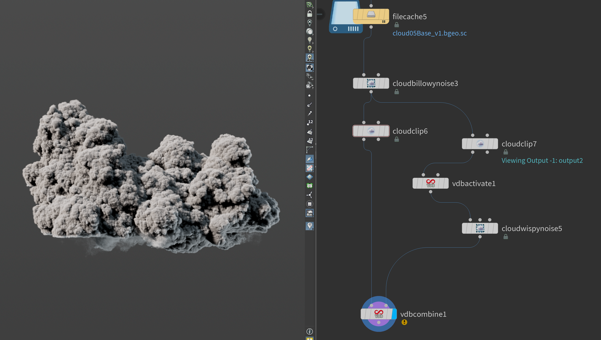
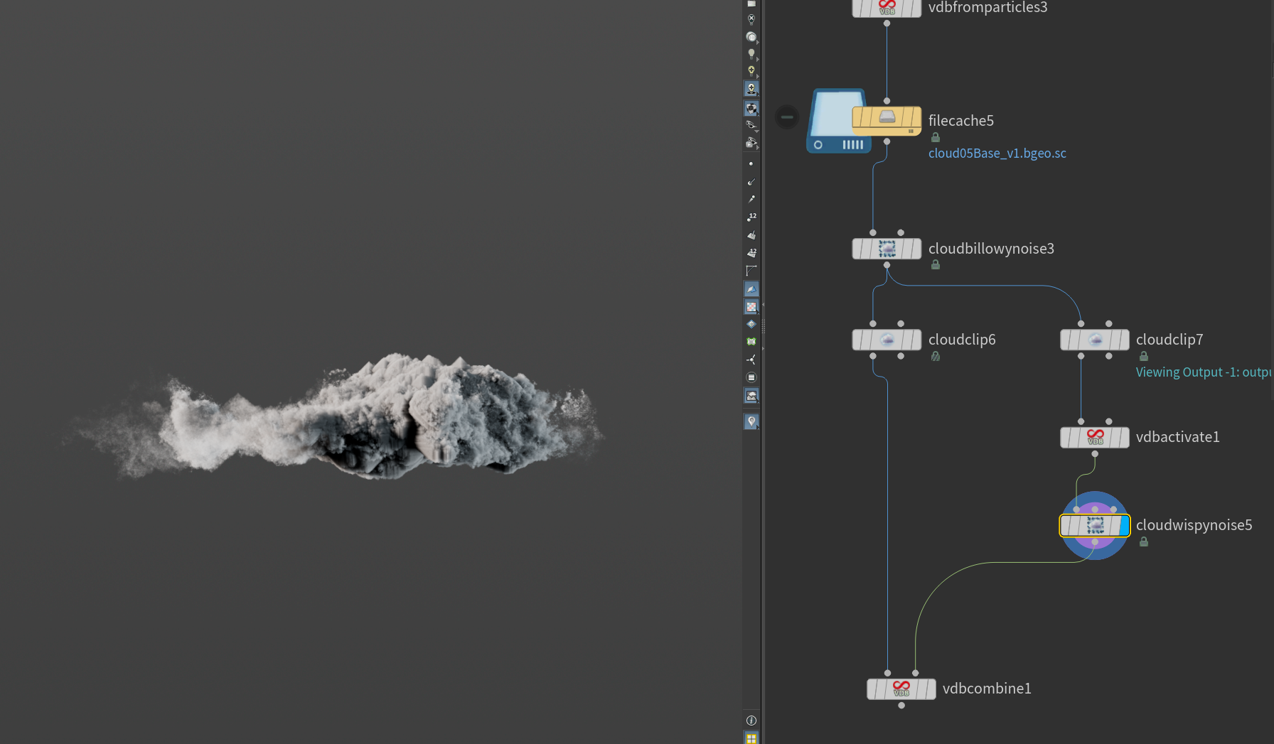
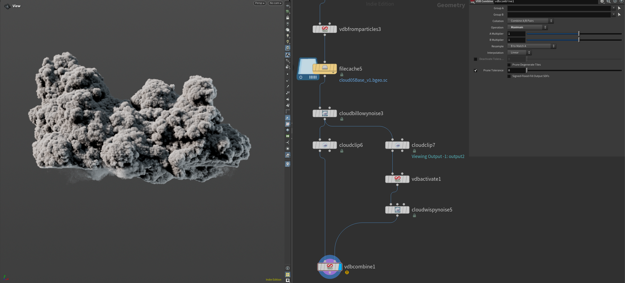
We're working with two streams - one for clipping the bottom of the cloud (left stream), and one for generating the wispy cloud formations near the bottom (right stream). We're then combining them both using a VDB Combine. I'll go into more detail on how this works, but I'll start by showing you the node network.
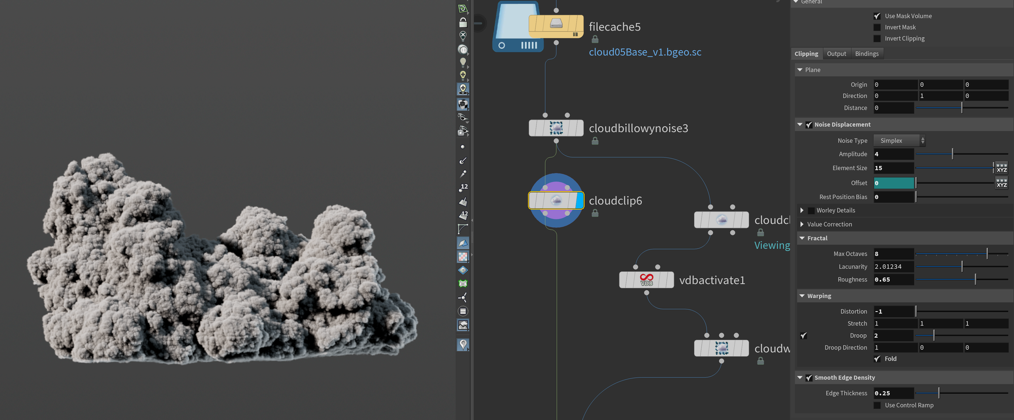
Let's start with the left stream. Here I generate the flat bottom for the cloud. I'm using mostly default settings, except I'm turning on Noise Displacement so the cloud bottom isn't completely flat. I'm also turning on Smooth Edge Density to soften the edges a bit as it can be a little sharp by default. Finally, I pipe all of this into the first input of the VDB Combine.
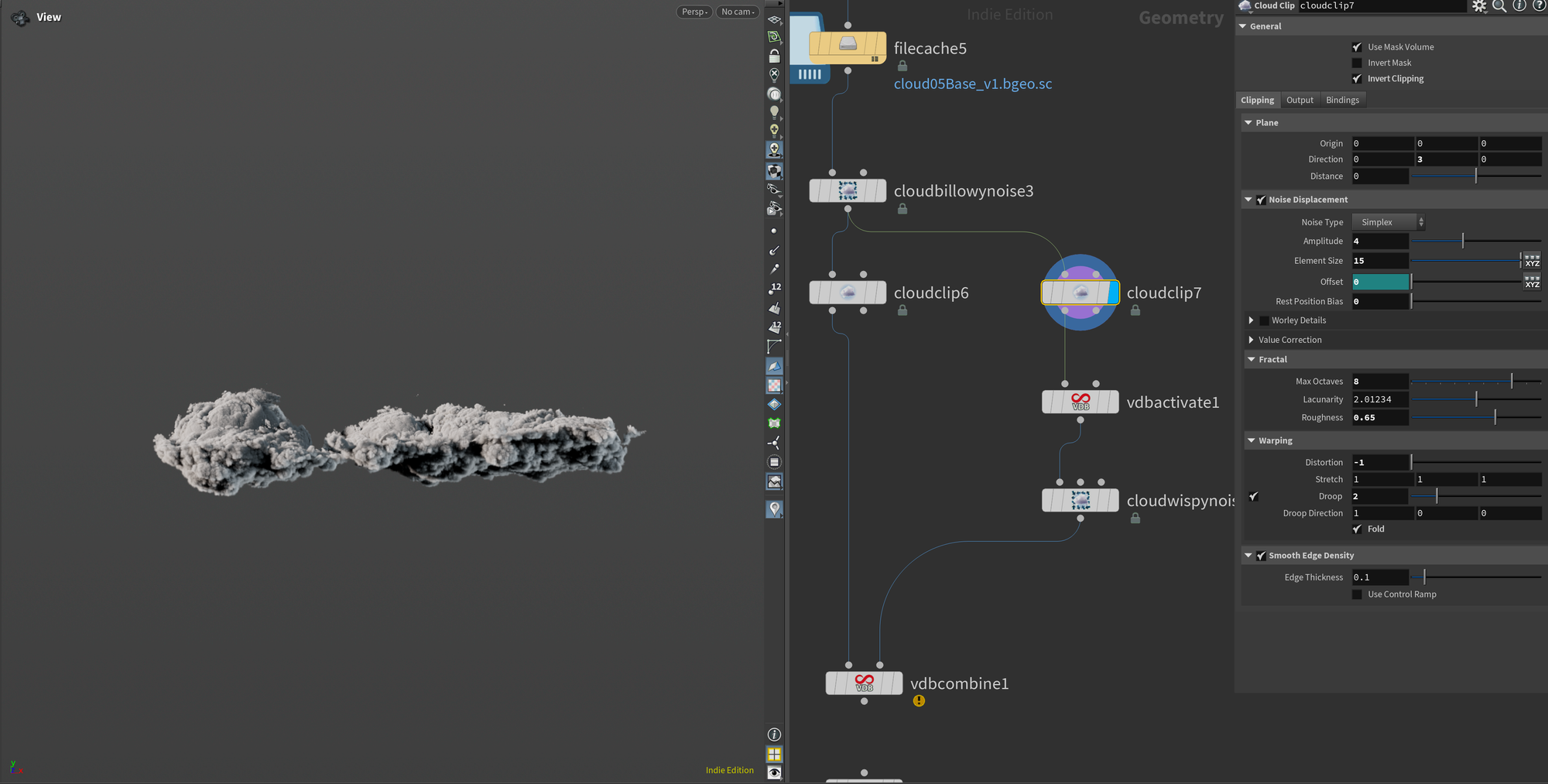
On the right side, things are a bit more complicated. First I copy the cloud clip from the other stream and adjust the direction a bit so it clips the volume further up (using the Direction parameter).
After that I enable Invert Clipping. This outputs the clipped part of the Cloud Clip SOP instead of the result of the clipping. We'll need this for creating our wispy cloud effect.
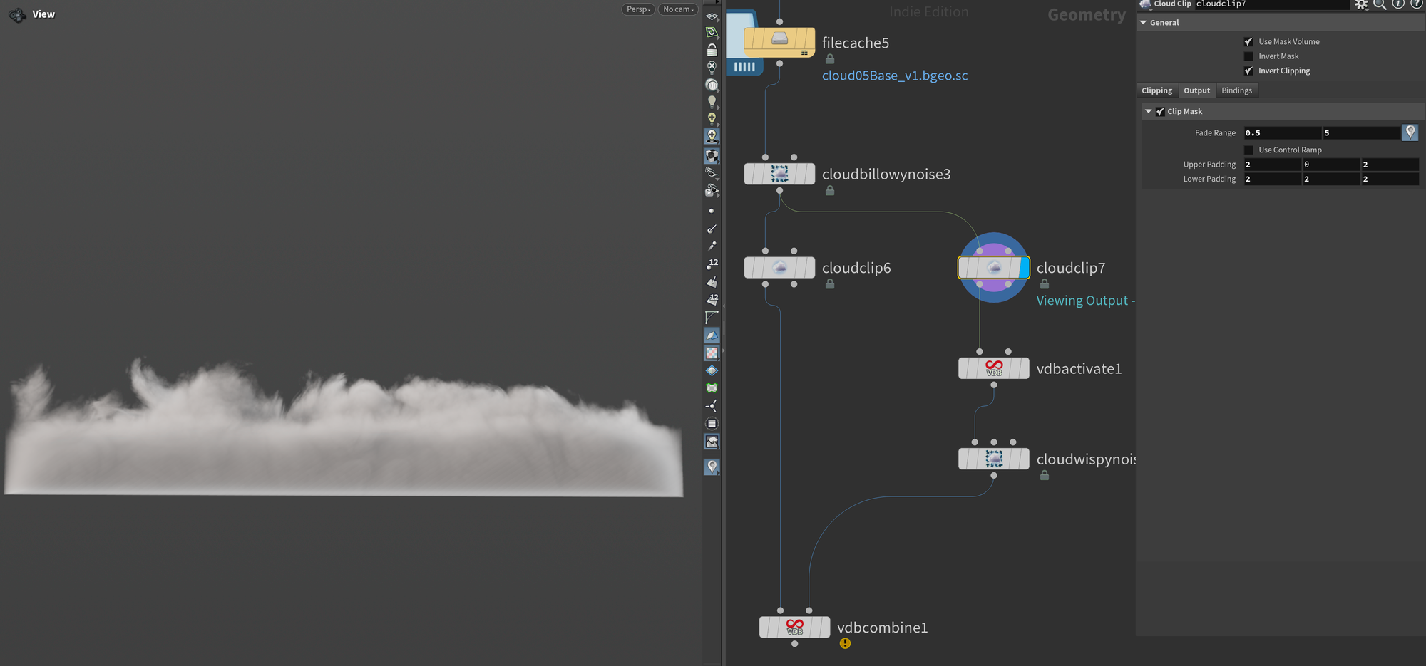
But that's not all, we're also outputting an extra volume called mask by enabling Clip Mask under Output (see the second image below). This will be used as a mask for the wispy noise node later. I'm also giving it a bit of extra padding so we have more area to work with as well as using Fade Range to soften it a bit so the cutoff isn't as sharp.
If you want to visualize the mask volume you can press the little "location marker" next to Fade Range.
After this node, I have a VDB Activate in my right stream. There's no real visual difference when you apply this node but it expands the active voxels, making sure that we have enough space for adding extra noise.
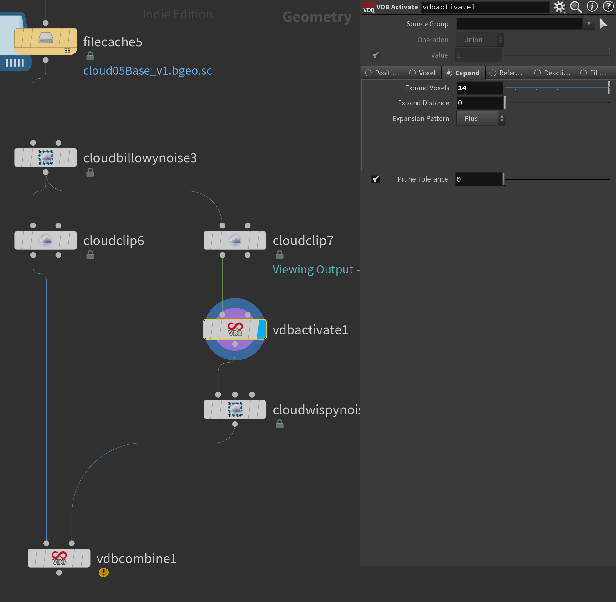
With our voxels activated, we can move on to making our bottom cloud part more "wispy".
For this, we'll use another node in the Houdini 20 cloud toolset called Cloud Wispy Noise.
We do need to adjust a few things in this node. First of all, we need to make use of the mask we generated earlier. To do this you simply enable Mask in the top of the node - this will pick up your mask volume and use it to mask the noise. I've also boosted the Amplitude quite a bit, adjusted the Roughness to 0.7 for more sharp displacement, and increased Substeps to 10.
In the Advection section, I enabled Advection and set the Noise Type to Zero Centered Perlin as I felt that gave me a more contrasty result.
Finally, in the Velocity section, I enabled wind - this helps give the noise a bit of direction - to simulate the lower parts of the cloud being affected more heavily by the wind.
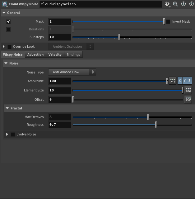
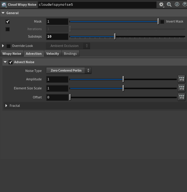
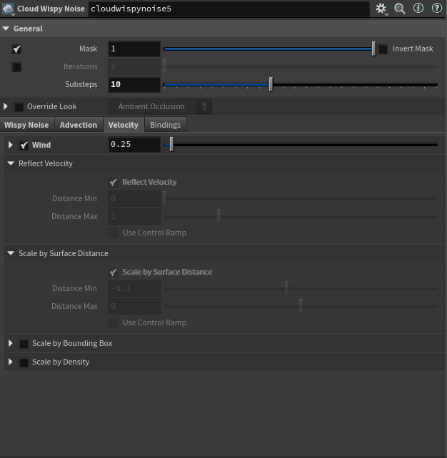
Cloud Wispy Noise settings
At the end of this chain, I combined both parts into one density volume using a VDB Combine set to Maximum. This effectively outputs the maximum value of any given area comparing two VDBs. This forms the final look of our cloud.
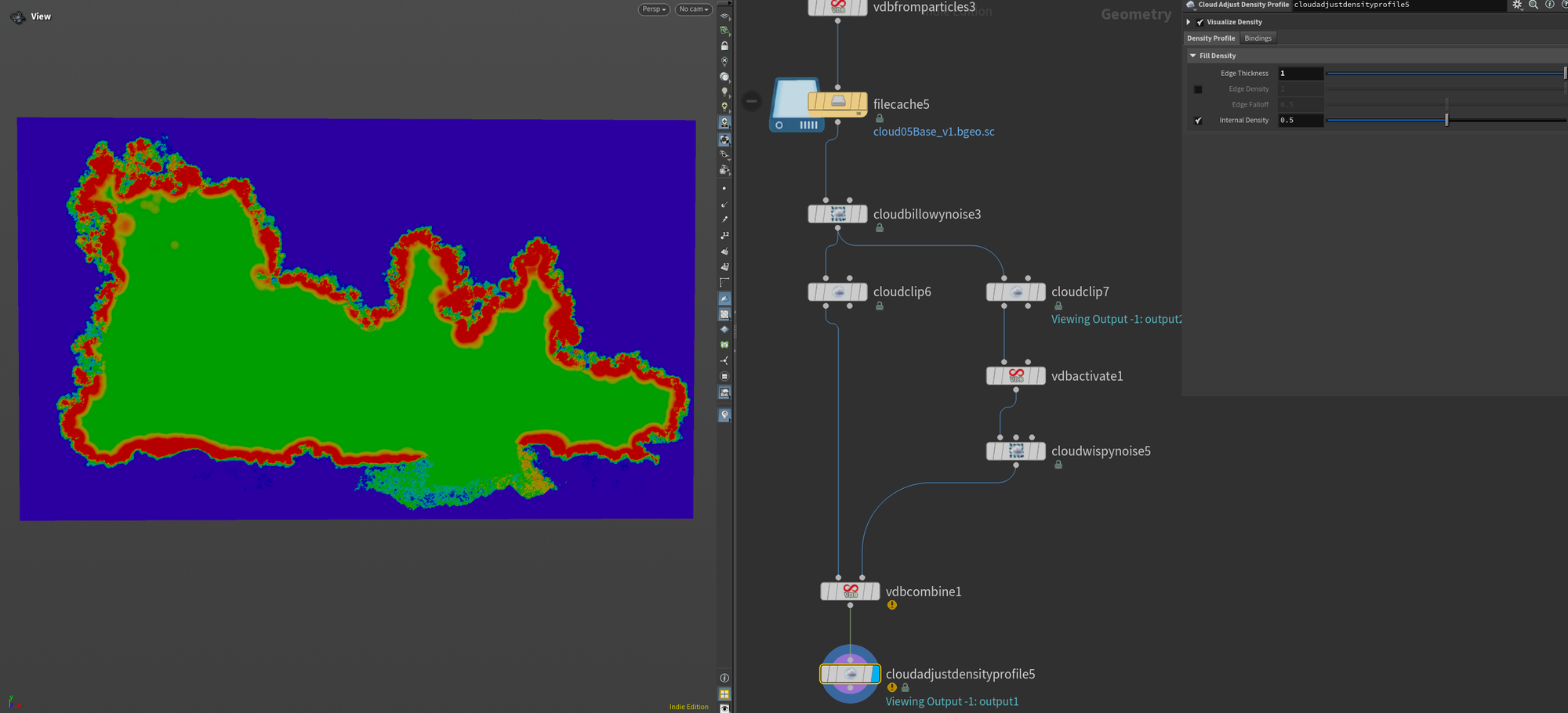
Cloud Adjust Density Profile
At the end of the chain, I tried playing around with a Cloud Adjust Density Profile. In this case, I used it to make the edge of the cloud thicker and lower the internal density. I felt this gave me a nice balance between scattering and shaping for the clouds. This node is something that I need to explore more, but I felt this setup worked well for my clouds.
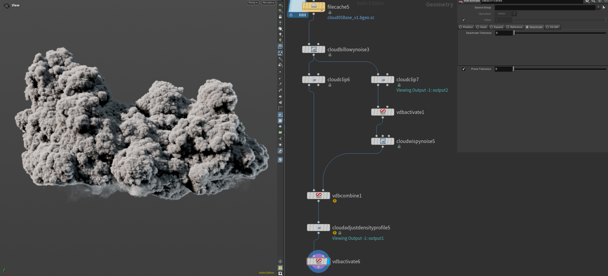
Final VDB Activate
To finish up our cloud I do a bit of optimization by making sure unused voxels are disabled (this goes back to the VDB feature of having inactive and active voxels that I mentioned before). If you switch the section to Deactivate it'll disable any voxels that have 0-values, which is what we want here.
Simulation
Custom cloud advection and lightning strikes
Custom Cloud Advection
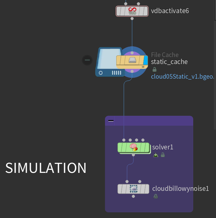
For this shot I wanted my clouds to have a subtle expansion to breathe some more life into them. I tried several different methods including a regular Pyro sim, but created my own simple SOP Solver instead since I wanted a very specific look.
I've outlined this setup below.
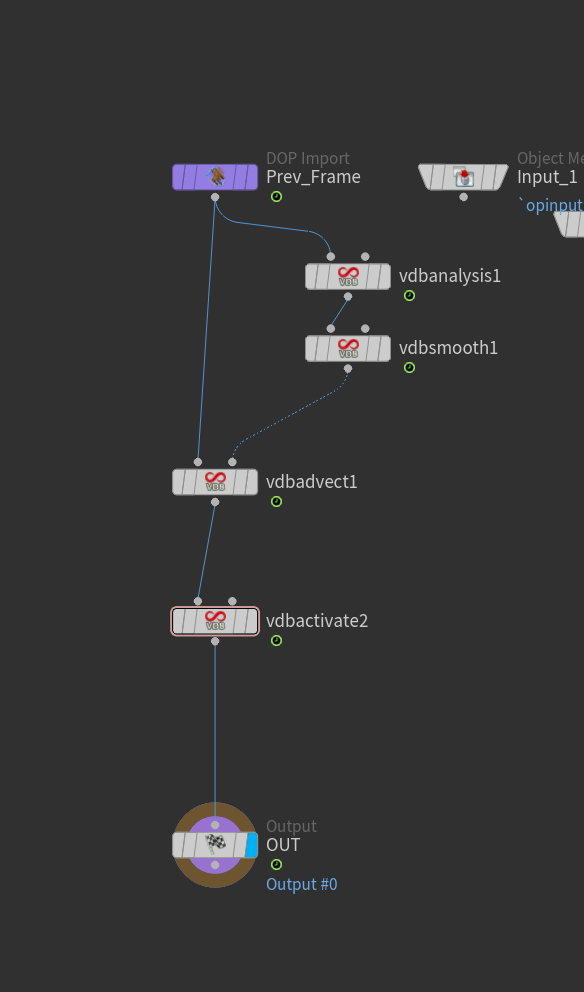
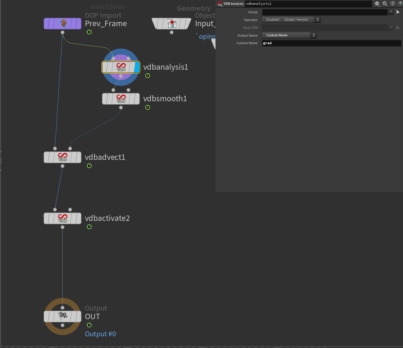
Let's go through what each node is doing and its parameters, starting with VDB Analysis. I'm using this node to generate a special Vector Field called Gradient. I name this custom field grad.
This is essentially the equivalent of normals but for volumes. It creates a vector field with voxels pointing in the direction of the "surface". As you might be able to imagine, this is the perfect field for creating controlled expansion as we can grow our volume "outwards" using this field.
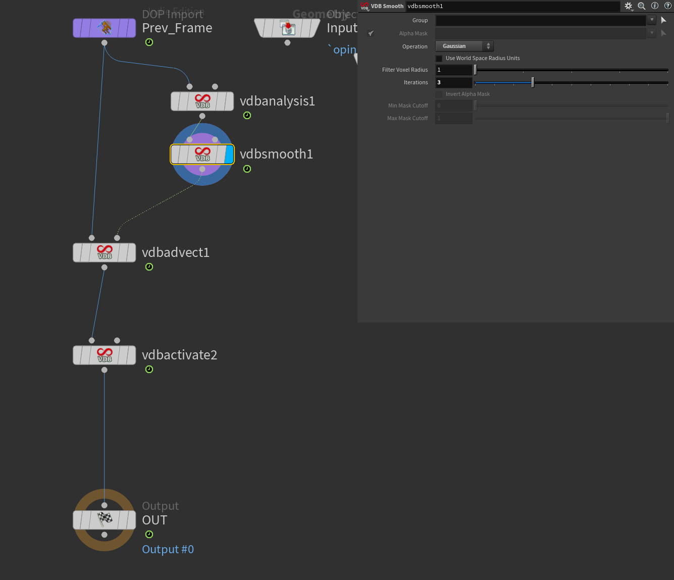
After this node, I chain a VDB Smooth which simply softens my Gradient field as I found the default Gradient field to be a bit too "choppy". I've set the iterations to 3 in my example, but you may have to dial this parameter in. Like most things surrounding simulation, it takes a bit of experimentation to get it right. Here I'm using the Gaussian operation for smoothing.
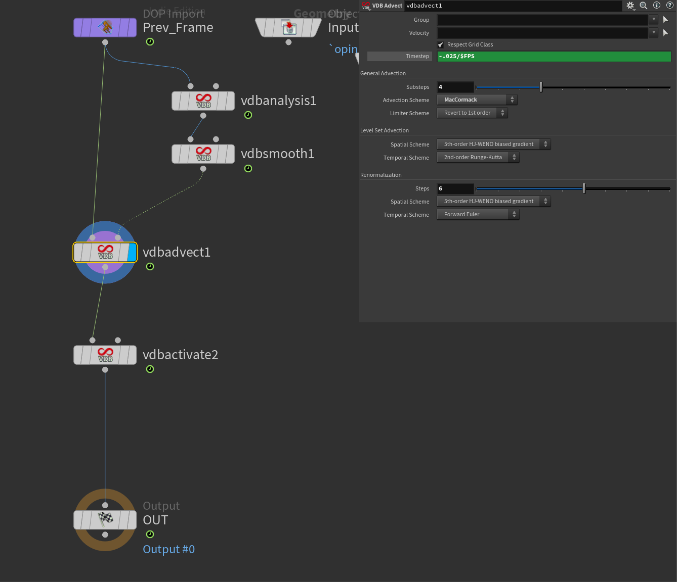
I then drop down a VDB Advect. This is our main driver for the simulation. This is the node responsible for advecting (or in more simple terms, expanding/moving) our voxels in the direction of the Gradient field.
In the first input, I plug in the Prev_Frame DOP Import, and in the second input, I plug in the result of my VDB Analysis + VDB Smooth stream.
I haven't modified too many parameters here, but let's go over the few that I have. First of all, I changed the Advection Scheme to MacCormack. I found this to give me the best results, and the default Pyro Solver uses a similar advection scheme. I also increased the Substeps to 4, and the Renormalization Steps to 6. Again these settings may take some dialing in for your cloud setup, but they should present you with a good starting point.
Most importantly here I divided the timestep to a very low amount. In my example, I've used -0.25/$FPS which gave me a good speed. This setting determines how much the volume should advect each frame. Notice the negative sign, if you don't use a negative sign your volume will expand inwards due to the nature of the gradient field.
This setting is likely what you'll end up spending the most time on. The lower the value, the slower it goes. So it might take a bit of time to find the right value. It's also very dependent on the resolution of the VDB, so if you increase resolution you may have to lower this as well.
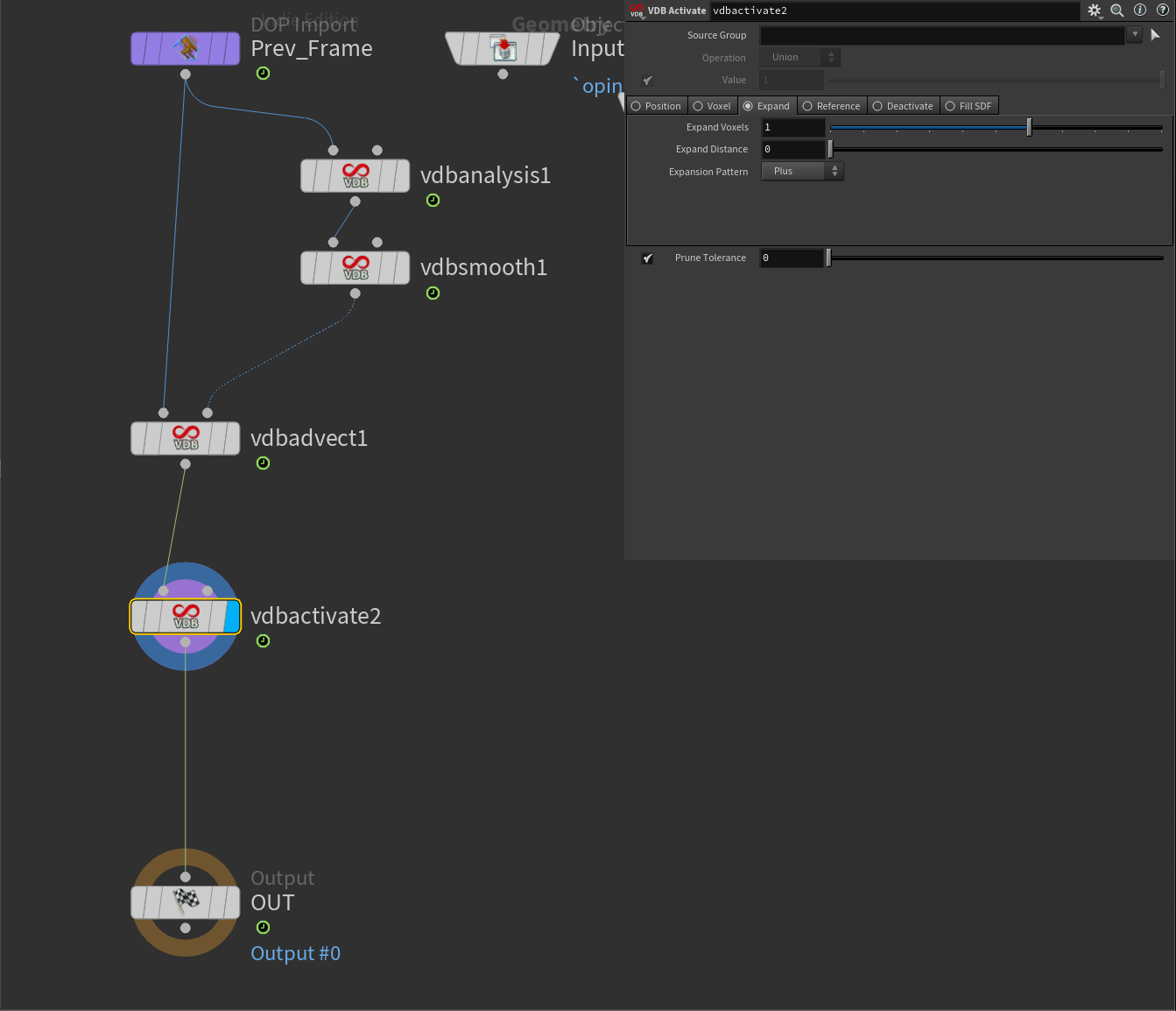
To finish our SOP Solver I added a VDB Activate at the end. This is very important as it expands the active voxel by 1. This makes sure that we have enough active voxels to perform our advection next frame. If you don't use this your density volume won't have enough room to advect and will look like a weird blocky volume.
Finally for our last step, I added a Cloud Billowy Noise after our SOP Solver (in the network outside) to add a bit extra detail. This is a static noise, but I found that it helps give a bit more detail since the advection does soften our volume a bit. In this case, I've also animated the Amplitude a bit so it's stronger towards the end of the simulation. I found that this gave the best look in my case, but your mileage may vary.
After this, I recommend you cache out your simulation using a Filecache node.
With that done we have our finished simulated cloud, ready for rendering! You can now duplicate this setup and create as many clouds as you want, modifying the parameters for each duplicate as you see fit.
Lighting & Shading
Custom cloud advection and lightning strikes
Now let's move on to Solaris. We'll revisit SOPs to generate a few things along the way, but for most of the remaining 3D section of this tutorial, I'll be working in Solaris.
Layout
First I want to import my volumes into Solaris and create a nice layout. Since I'm dealing with a small amount of clouds for this shot I've skipped the process of generating proxies - if you want to learn about that check out my previous tutorial Creating Procedural Drift Ice in Houdini using SOPs and Solaris.
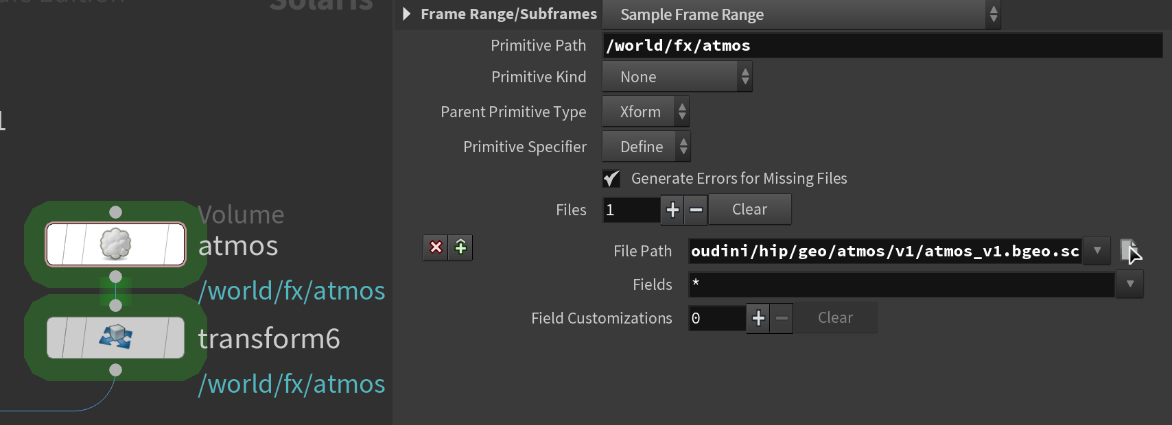
Layout in this case was pretty simple. I loaded each cloud into the /stage context using Volume LOPs. For the Primitive Path I set it to a path structure I liked (I like to organize things by /world/<department>/<assetName>/<primName> but it's completely up to you. You can see an example below.
One interesting thing to note is that you can load bgeo.sc files directly into the Volume LOP. It works just like .vdb files. I haven't tested if this is more or less performant, but I thought it was neat that it was possible.
Underneath each of these Volume LOPs, I added a transform node - this is the node I use to modify the placement of each cloud.
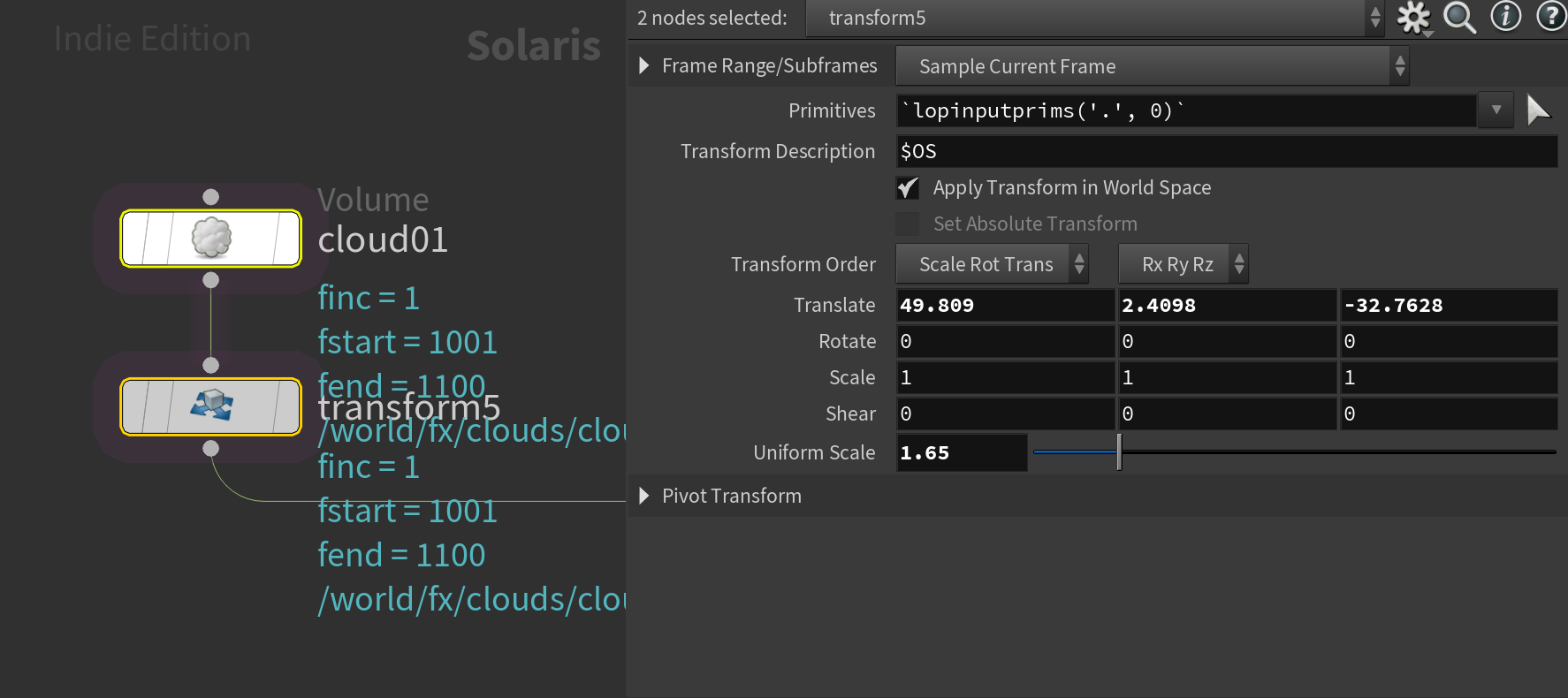
You can see it worked if there's no "clock" icon next to your nodes.
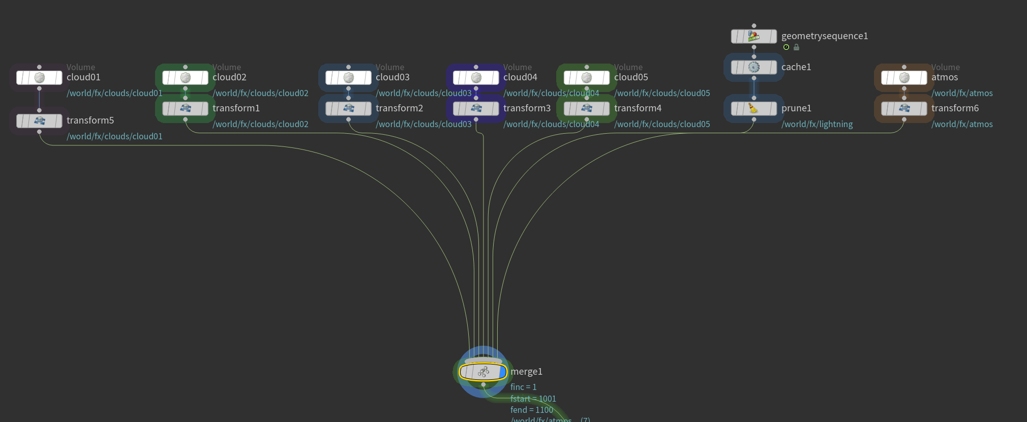
In the end, all of the different transforms go into one merge node. Please ignore the 2 nodes at the edge of this network (geometrysequence1 and atmos - I'll cover these later.)
Lightning Strikes
For the lightning strikes in this shot, I wanted something fairly simple. My goal was just to have them turn on and off on a couple of random frames (I ended up extending this slightly in comp, but more on that later).
I knew I wanted to base the lightning strikes on my cloud models, having some of them inside the clouds and others outside.
To do that I imported the layout I created into SOPs and used a scatter node to scatter a bunch of points inside the clouds.
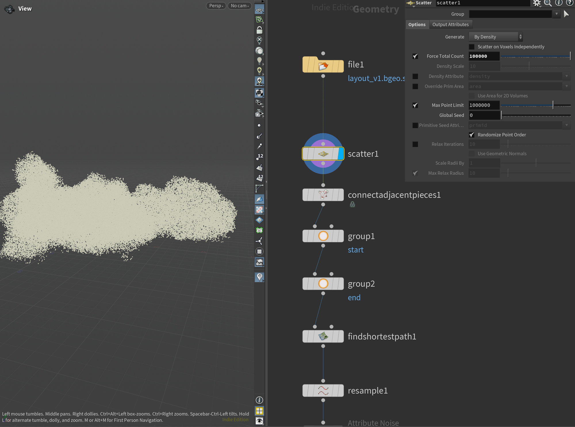
After that, I connected all the points using Connect Adjacent Pieces. This will be the base for our lightning geometry.
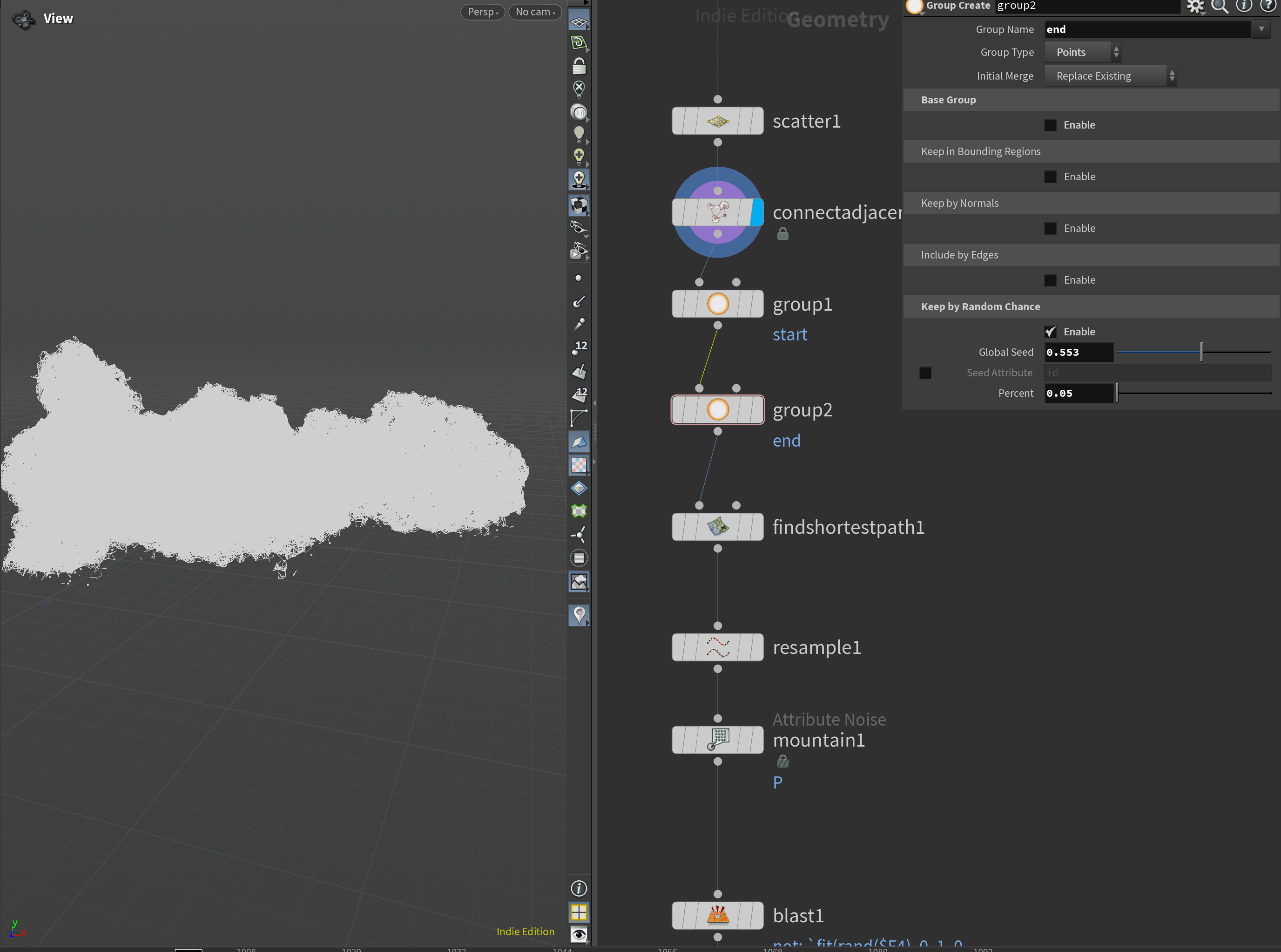
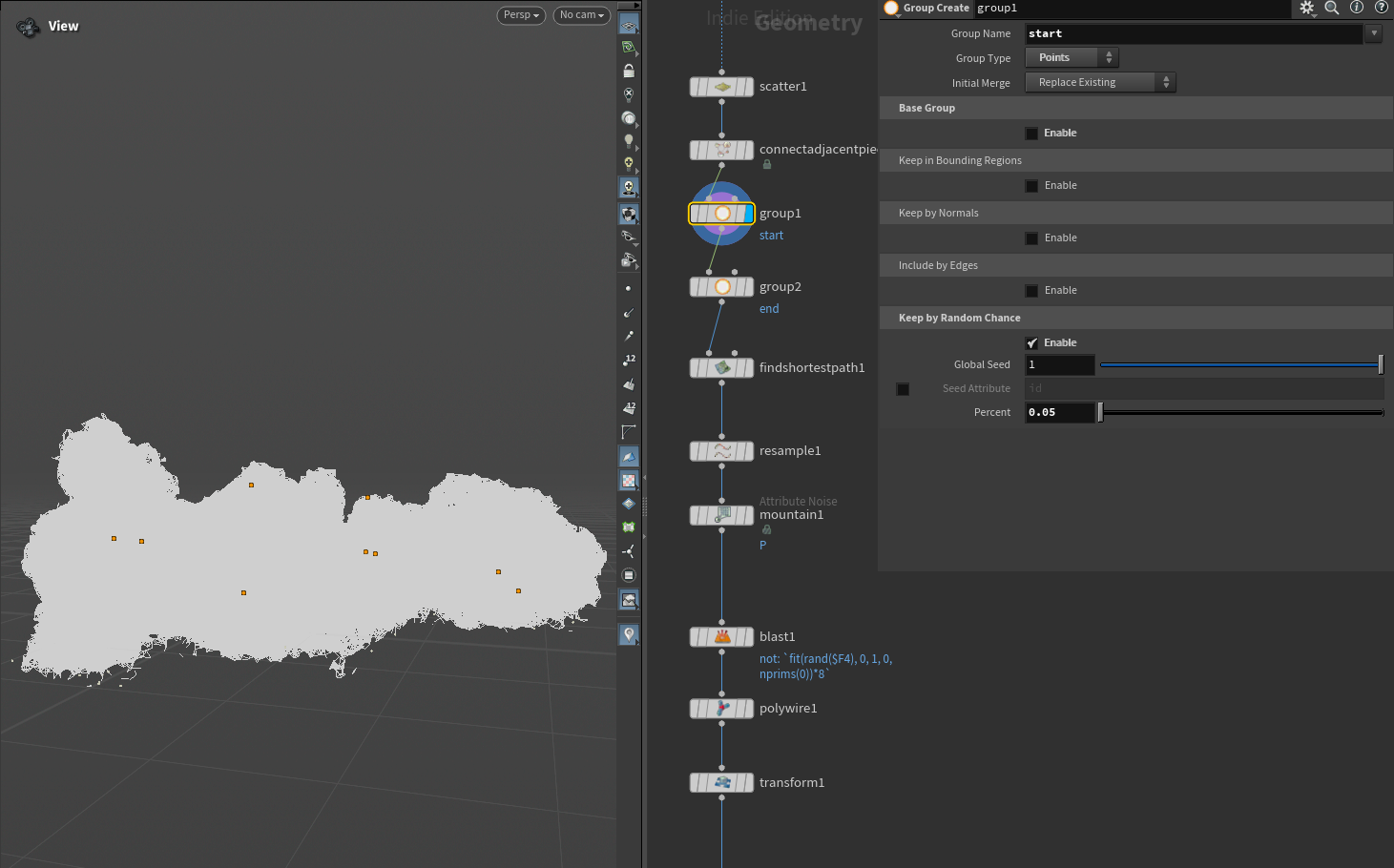
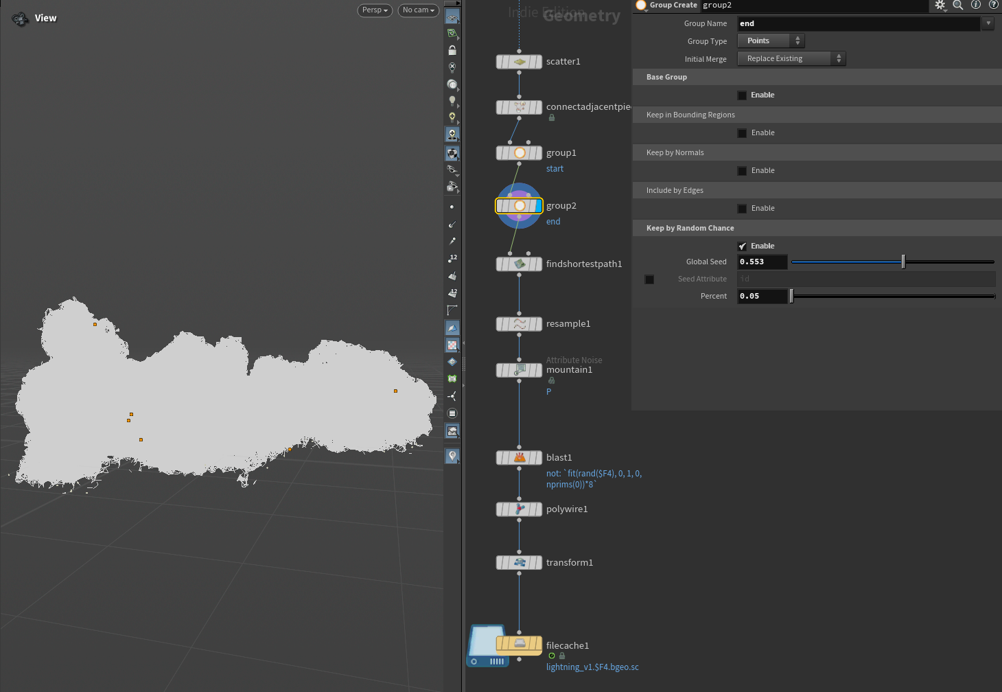
After this, I created two groups - start and end. I did this using a group node set to Points with Keep By Random Chance enabled. I only wanted a very small amount of points so I kept the percentage low. These will be the start and end points of our procedurally generated lightning strikes.
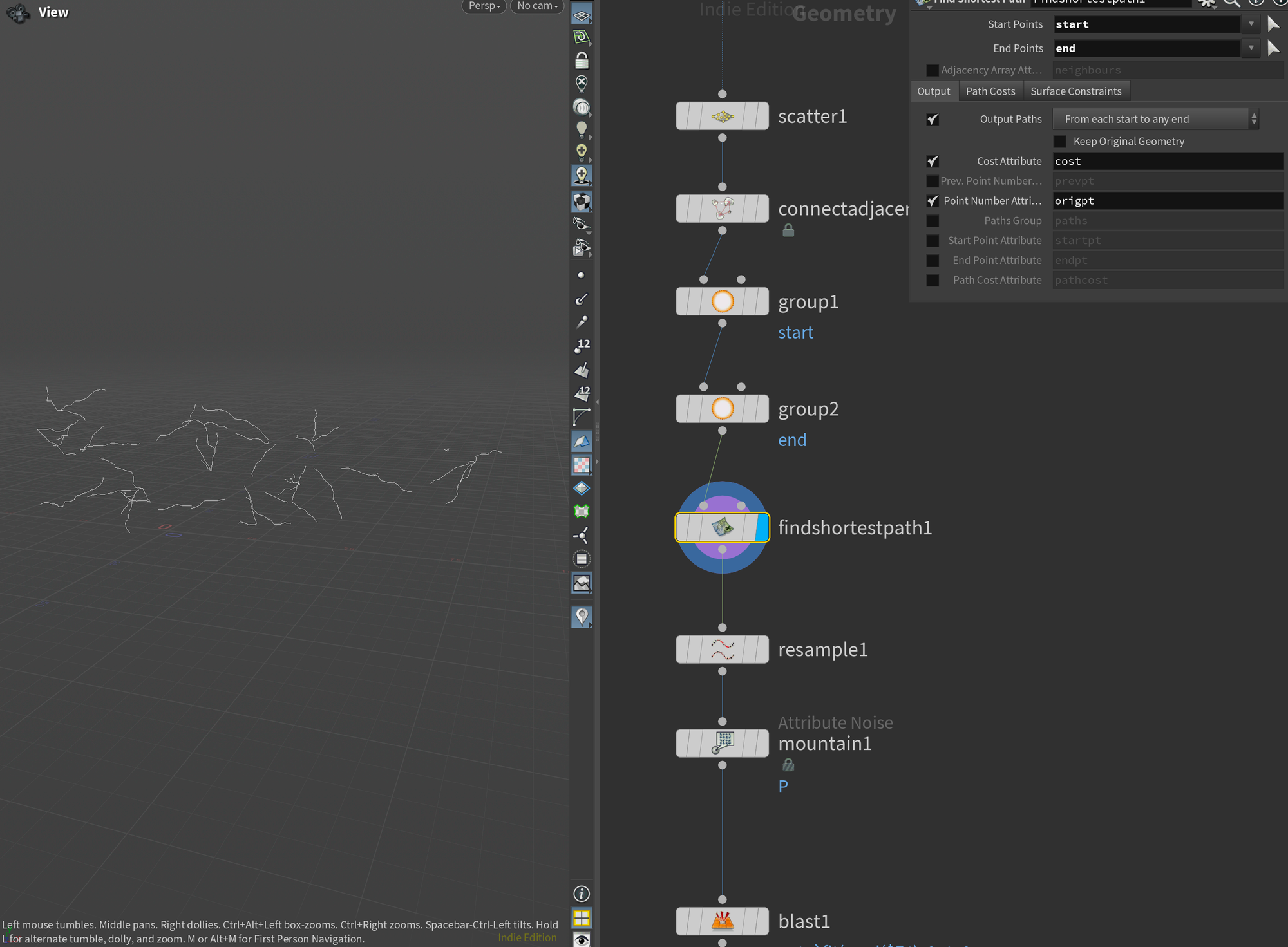
And now for the meat of our lightning generator. I appended a Find Shortest Path node to my network. This node does more or less what it says. I plug in my start and end group - the node will then try to find the shortest path to the corresponding endpoint.
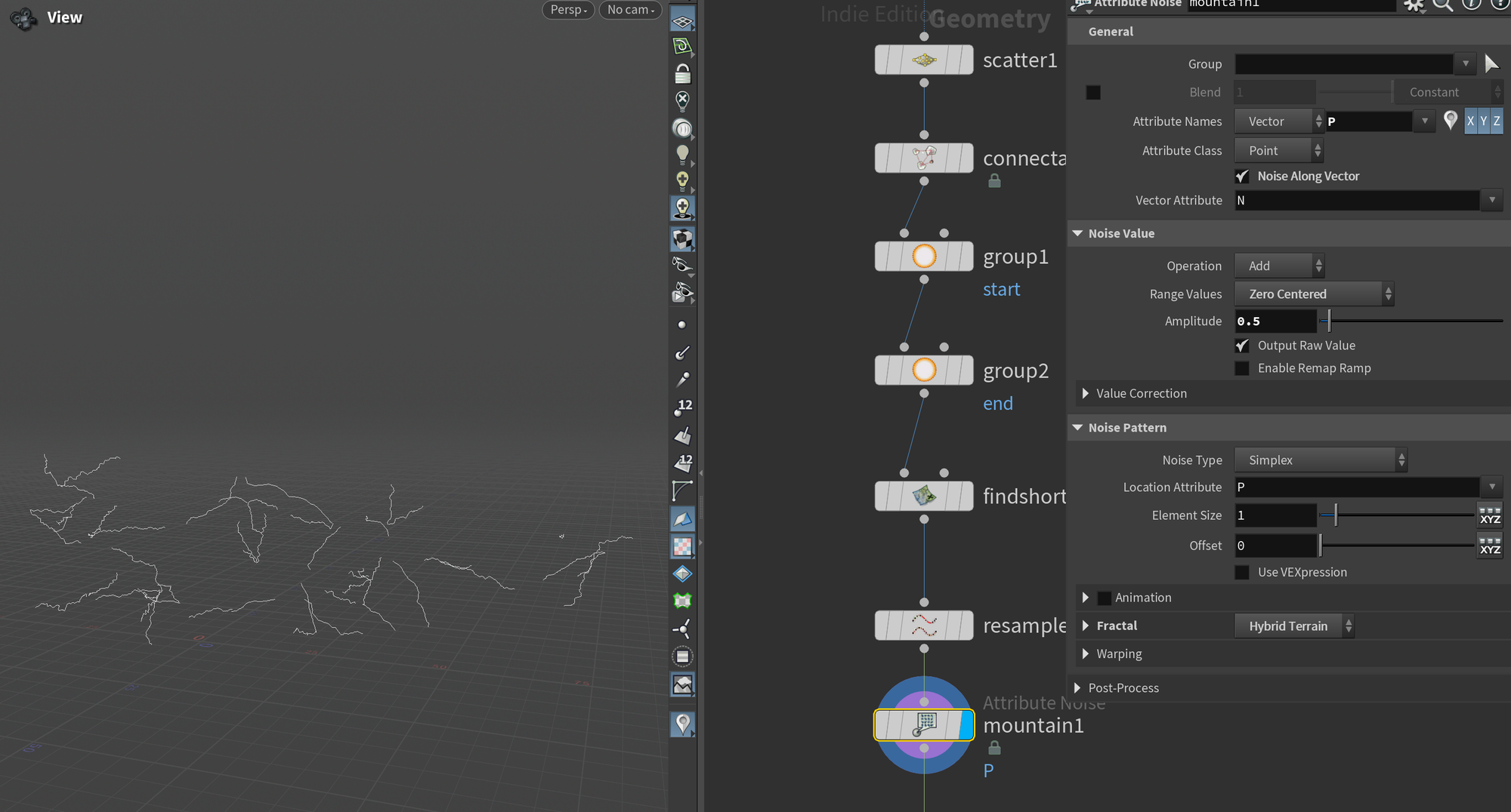
The lighting was a bit too smooth, so I added a Resample node to get more points, followed by a Mountain SOP to create some more noise.
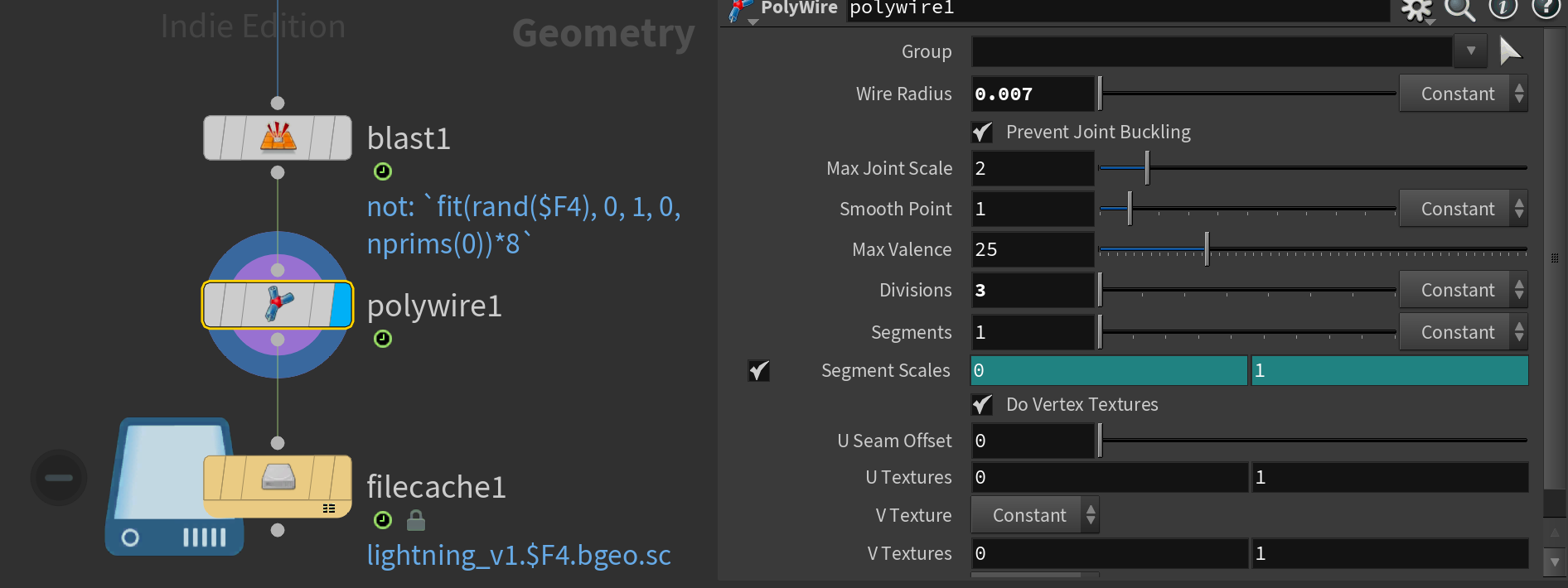
Now let's animate the lightning strikes! I did this using an expression in a Blast SOP set to Primitives:
`fit(rand($F4), 0, 1, 0, nprims(0))*8`This will randomly assign a number between 0-1 to each primitive (lightning strike), fit it between 0 and the number of prims (lightning strikes), and then multiply it by 8.
This will make it so the lighting strikes will randomly turn on and off for each frame. The last integer in the expression (8) is what controls the frequency of the lightning strikes appearing. Higher values correspond to higher frequency, lower values correspond to lower frequency.

At the very end after all of this, I add a Polywire SOP with an appropriate Wire Radius, and finally add a File Cache to cache the whole frame range for rendering.
In Solaris, I load this .bgeo.sc file using a Geometry Sequence LOP. I set the Import Path Prefix to something appropriate for the scenegraph setup I have and set the Topology Attributes parameter to Animated since we have an animated topology.
I then append a Cache LOP set to Always Cache All Frames to force Solaris to write USD Time Samples and remove time dependency - improving our cooking time.
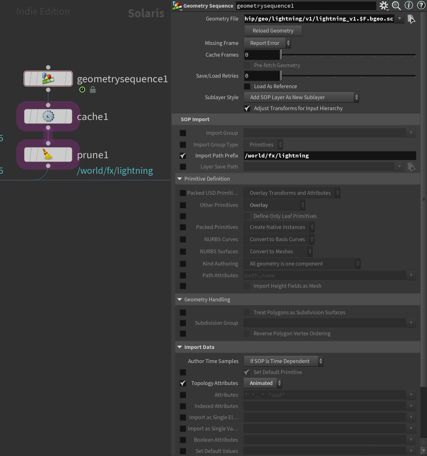
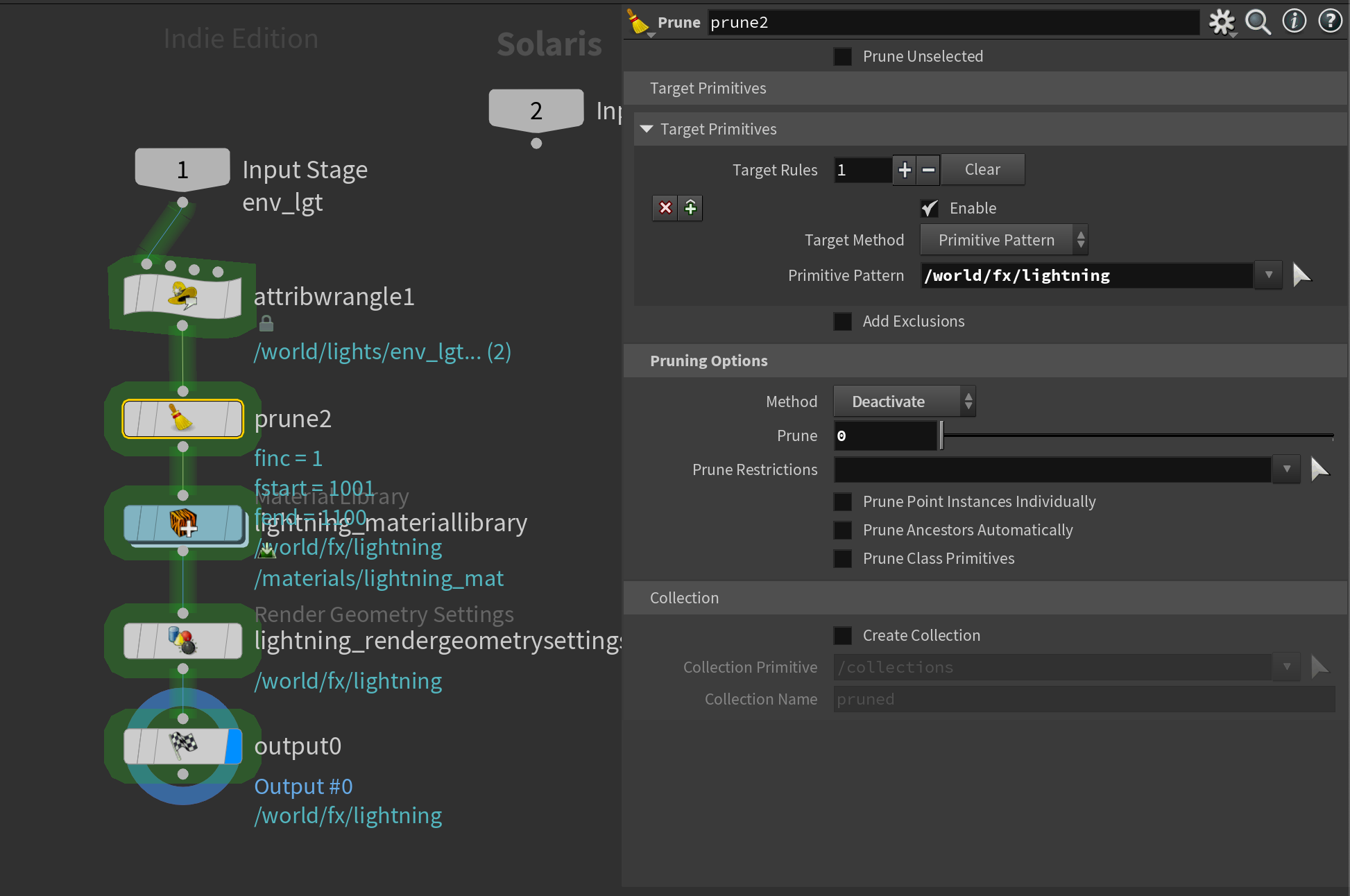
You'll notice I also added a Prune LOP here. I use this to disable the lightning primitive by default so I can enable it only on my lightning render layer later.
Atmosphere
One final addition to our setup is a bit of atmosphere. I wanted to add a gradient of an atmosphere coming from the bottom of the screen and slowly fading out towards the bottom third of the screen.
I created this by appending a box roughly in the size I wanted the atmosphere to be (I'll transform this more in Solaris later). I then turned it into a Fog VDB using a VDB From Polygons.
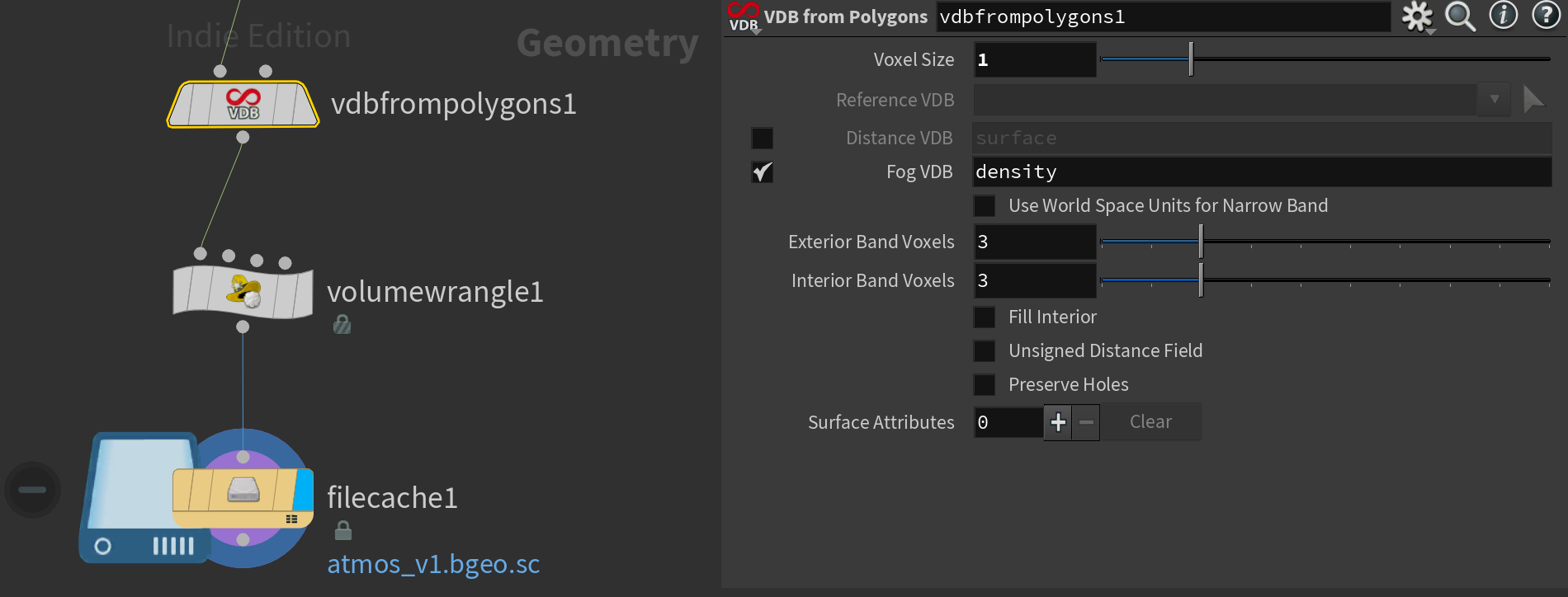
I then added a Volume Wrangle with the code below. Remember to click "Generate Spare Parameters" as the code creates the spline ramp you see below.
The code essentially creates a ramp and multiplies it with the density. The ramp is based on the position of the Y min and max of the bounding box (computed using the getbbox_max and getbbox_min functions).
f@density *= chramp("gradient", fit(@P.y, getbbox_max(0).y, getbbox_min(0).y, 0, 1))*.01;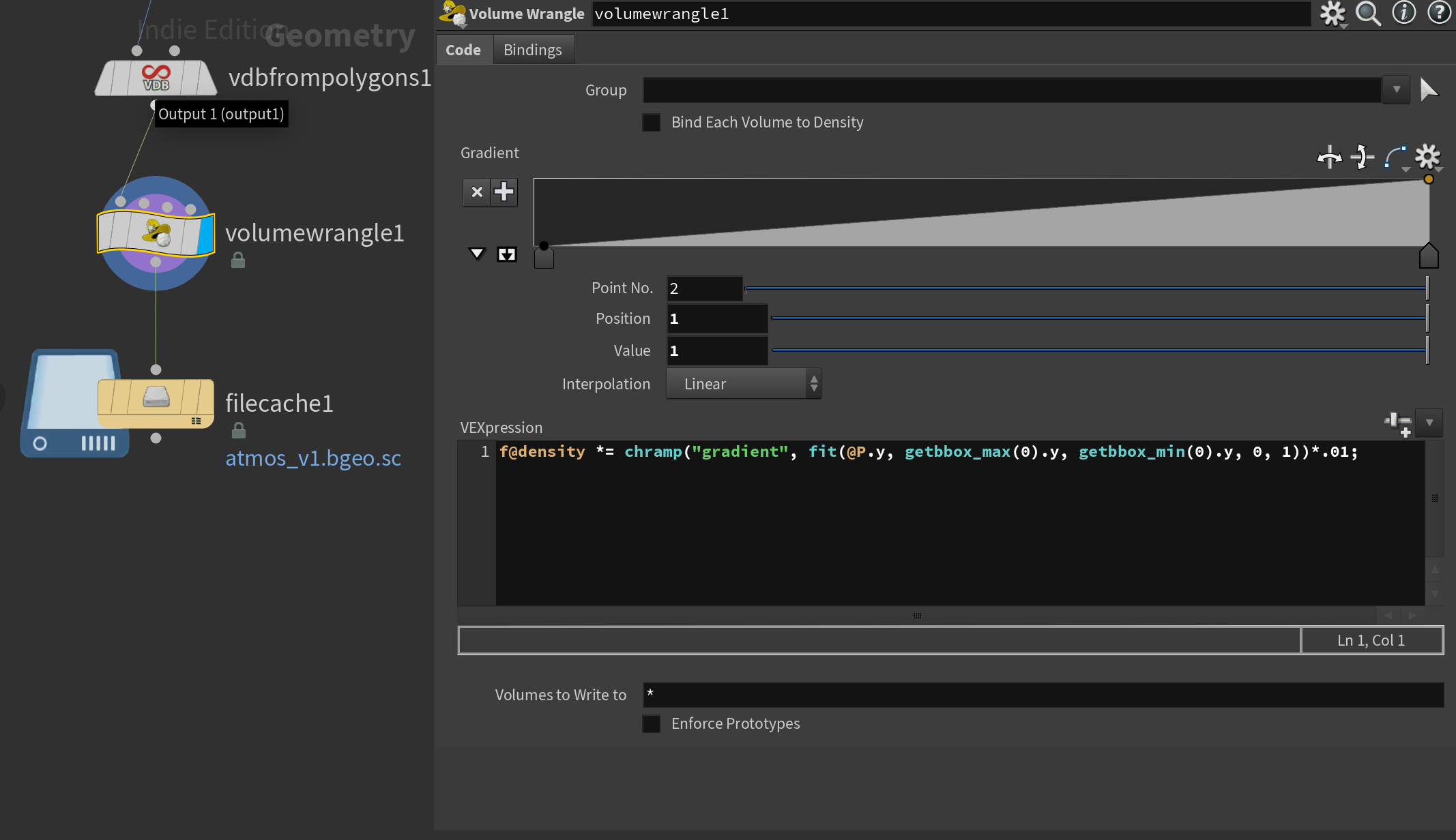
As always I then export the output of this using a File Cache.
When importing this into Solaris I use the same approach as I did for my clouds, simply loading it using a Volume LOP and appending a transform to scale it a bit to my liking.
Shading
Cloud Shader
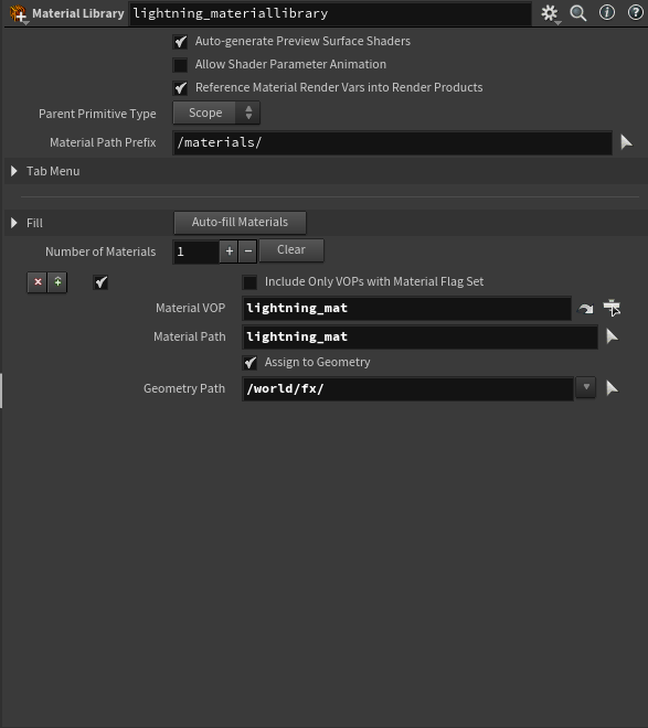
Now let's move on to shading! I'll start by looking at how I approached shading our clouds. All of the shaders were built and assigned using a Material Library LOP.
For the cloud shader, I used the cloud shader preset included in Houdini 20 as I liked the results it delivered. You can access this through the Tab-menu searching for "Karma Cloud Material".
The only thing I adjusted here was the Density Scale and enabling the Use Secondary Anisotropy toggle. The Secondary Anisoptropy helps add a bit of shaping to the clouds, otherwise, I find that a lot of details are lost to the multi-scatter effects.
Atmosphere Shader
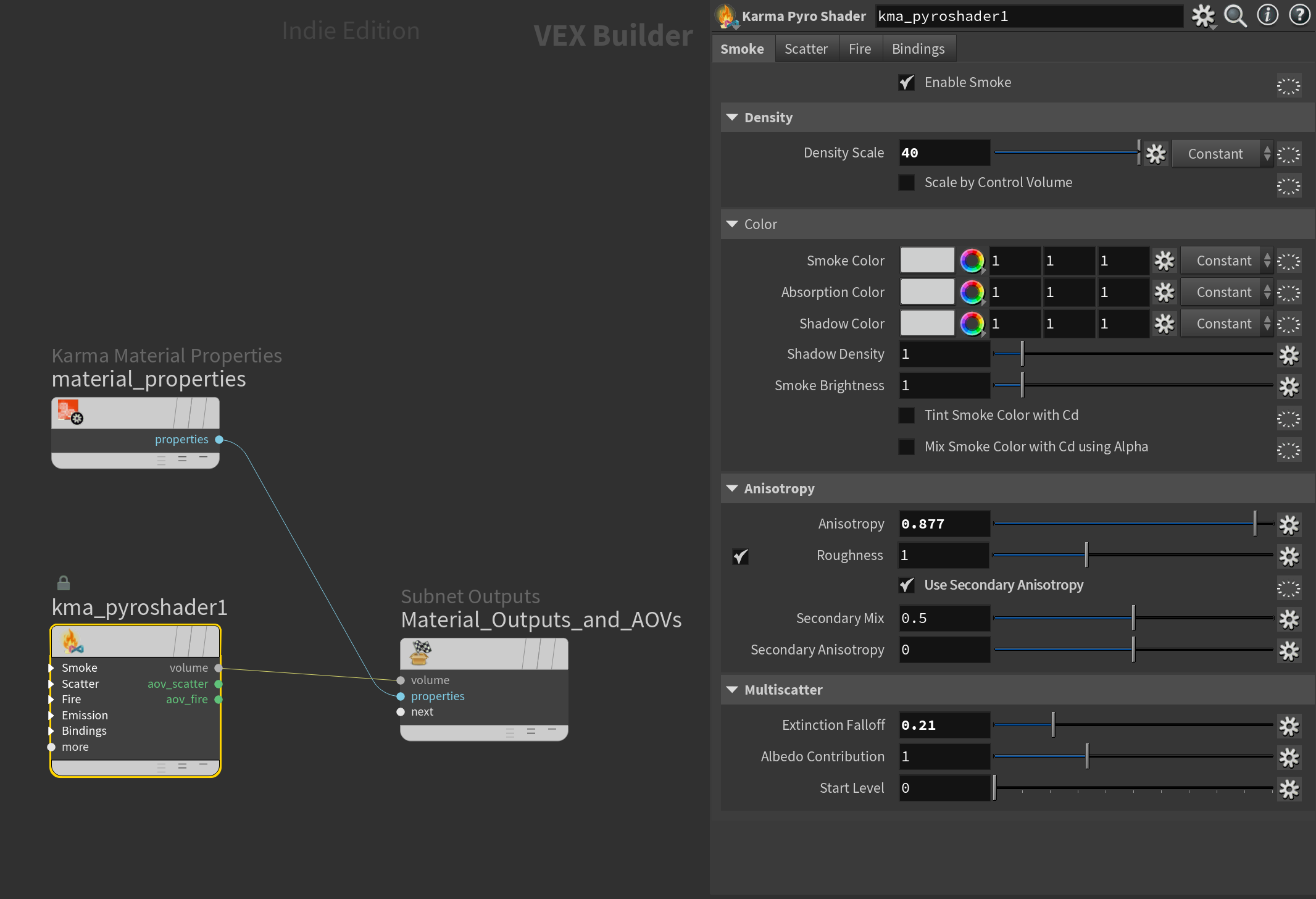
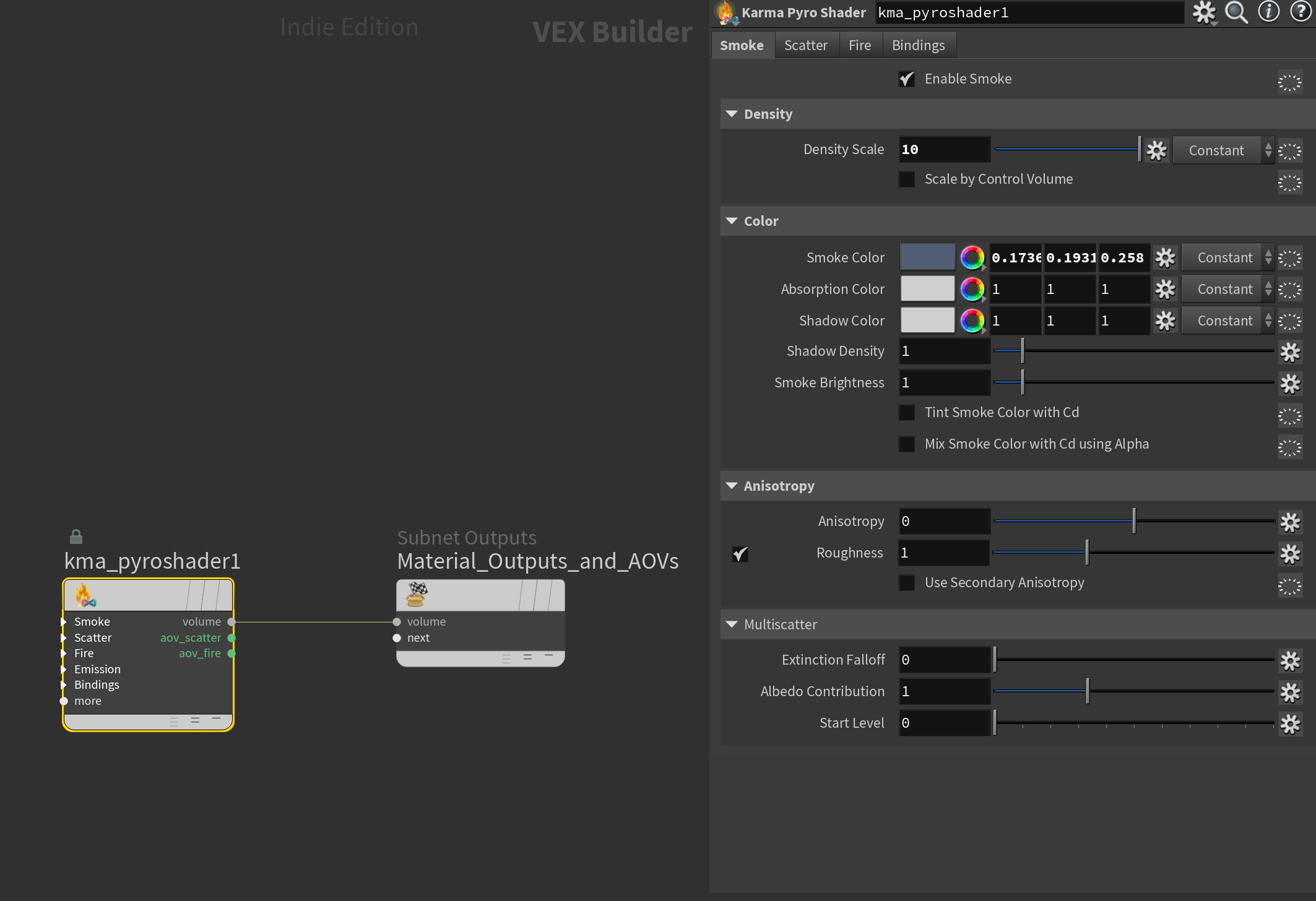
For the atmosphere I created a Karma Material Builder, dived inside, and replaced everything with a single Karma Pyro Shader plugged into the material output. This shader is very simple, I adjusted the smoke color to be a dark blue (as I wanted this to work as a dark gradient going from the bottom of the screen to the bottom third) and boosted the density as I saw fit.
Lighting
For the lighting, I'm going to split the tutorial into two sections - the beauty render layer and the lightning render layer. This is because I rendered the cloud beauty and lightning render separately to have more flexibility in compositing. Let's start with the beauty!
Beauty Render Layer
The beauty consists of the clouds, atmosphere, and two lights.
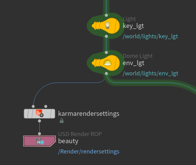
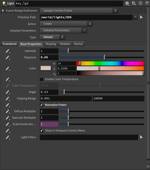
For the key light, I added a simple Distant Light with a light pink color to it and rotated it until I got some nice backlighting similar to the color you may get right around dusk.
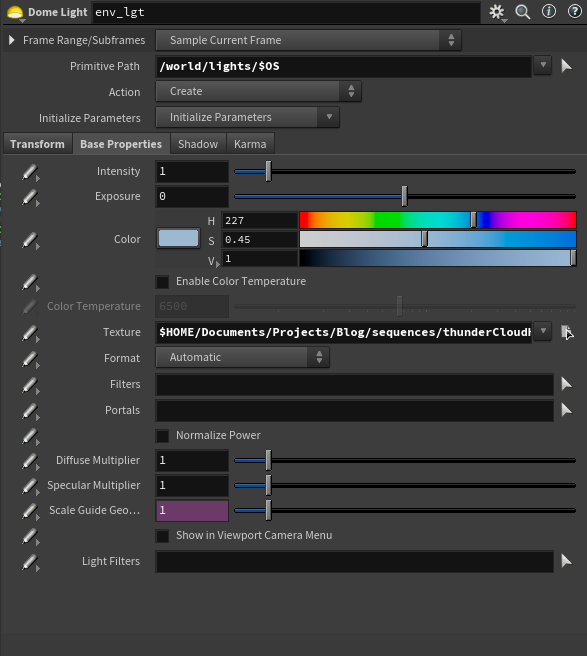
For the environment light / fill I added a Dome Light with an HDRI of a night sky from Poly Haven. I then tinted it using the Color attribute to get it a bit more blue. If you change the color in the dome light while you have an HDRI plugged in it will multiply that HDRI by that color.
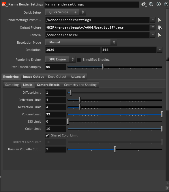
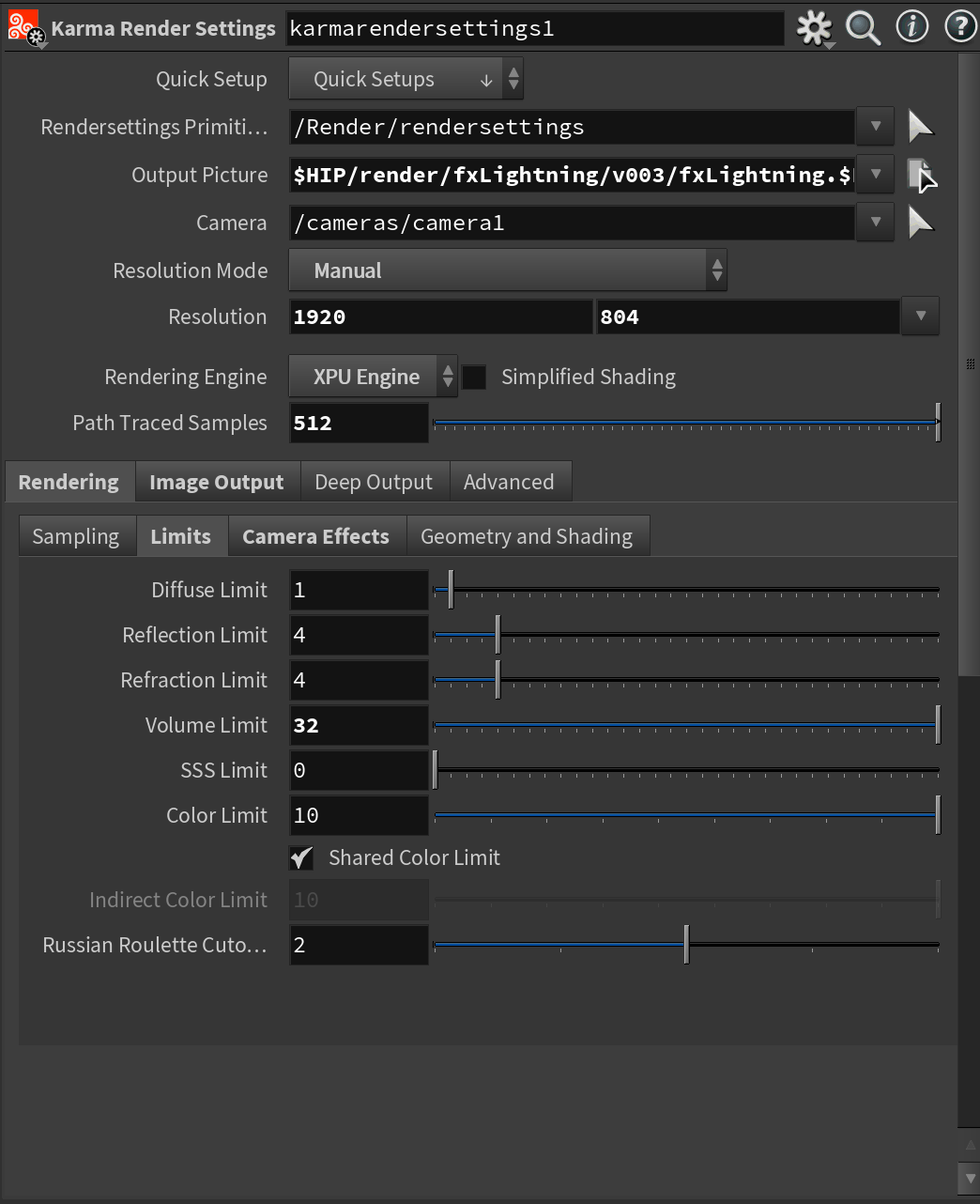
For the render settings, I set the Render Engine to use XPU as I found it significantly faster for this - even without an RTX card. I rendered this shot on a Mac Studio with an M2 Ultra chip.
Most importantly here I dialed in the Volume Limit to 22. It is necessary to set this value relatively high to get proper scattering from the cloud shader. So if your cloud looks odd take a look at this setting.
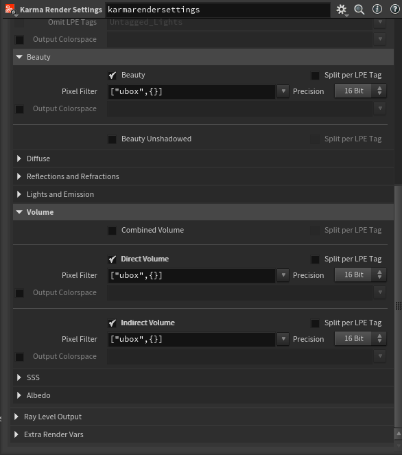
Finally, for the AOVs (in the Image Output section) I output Direct Volume and Indirect Volume. This will get us the direct lighting and scattering separately for the clouds. Later in comp, this will become very useful.
After this, I appended a USD Render ROP and rendered out the sequence. Beauty done!
Lightning Render Layer
Since I wanted the lightning layer as a separate layer for more control in comp, I created a second stream just for that.
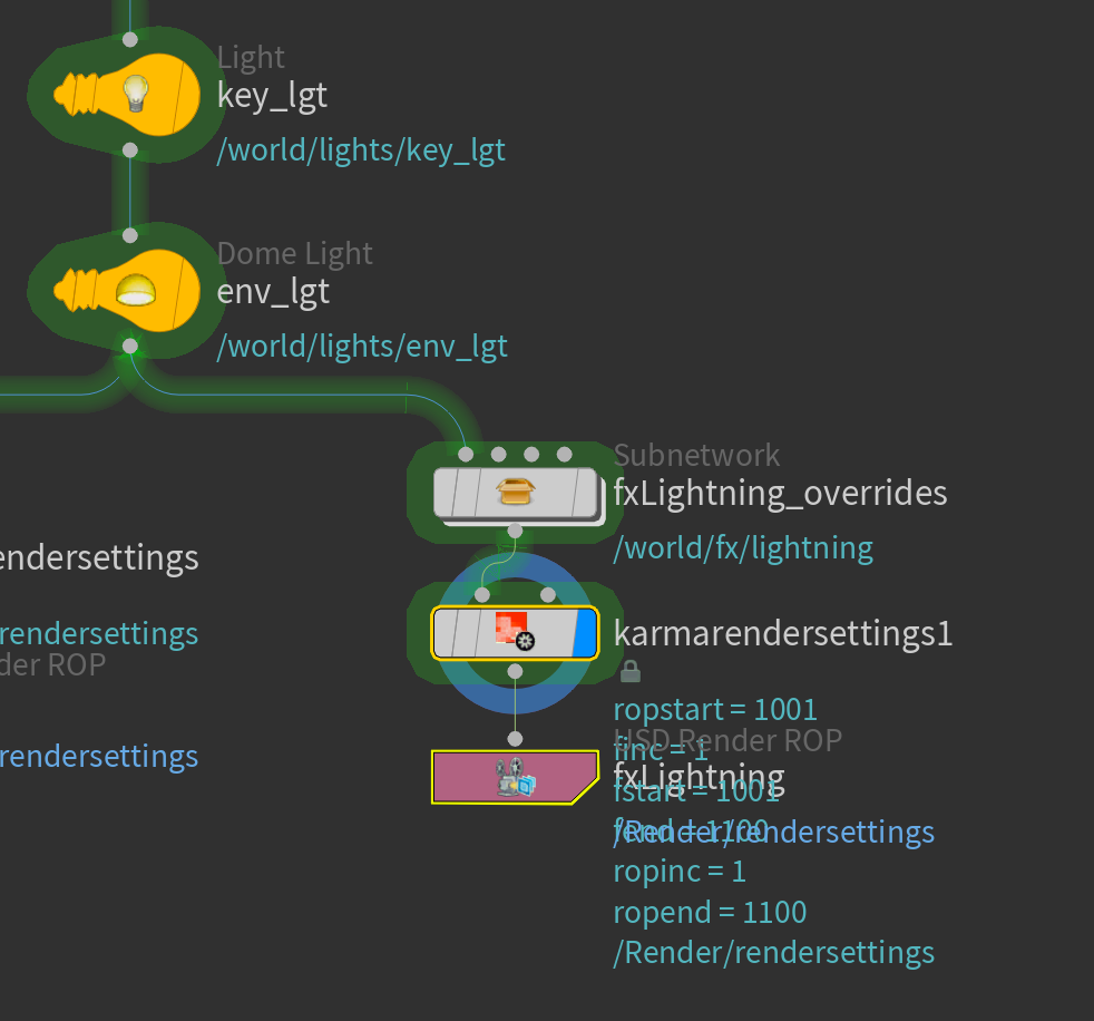
The meat of the setup is inside my fxLighting_overrides subnetwork. I like to split my setups into little modules like this - I find it gives you a better overview of the node network. Let's jump inside the subnetwork.
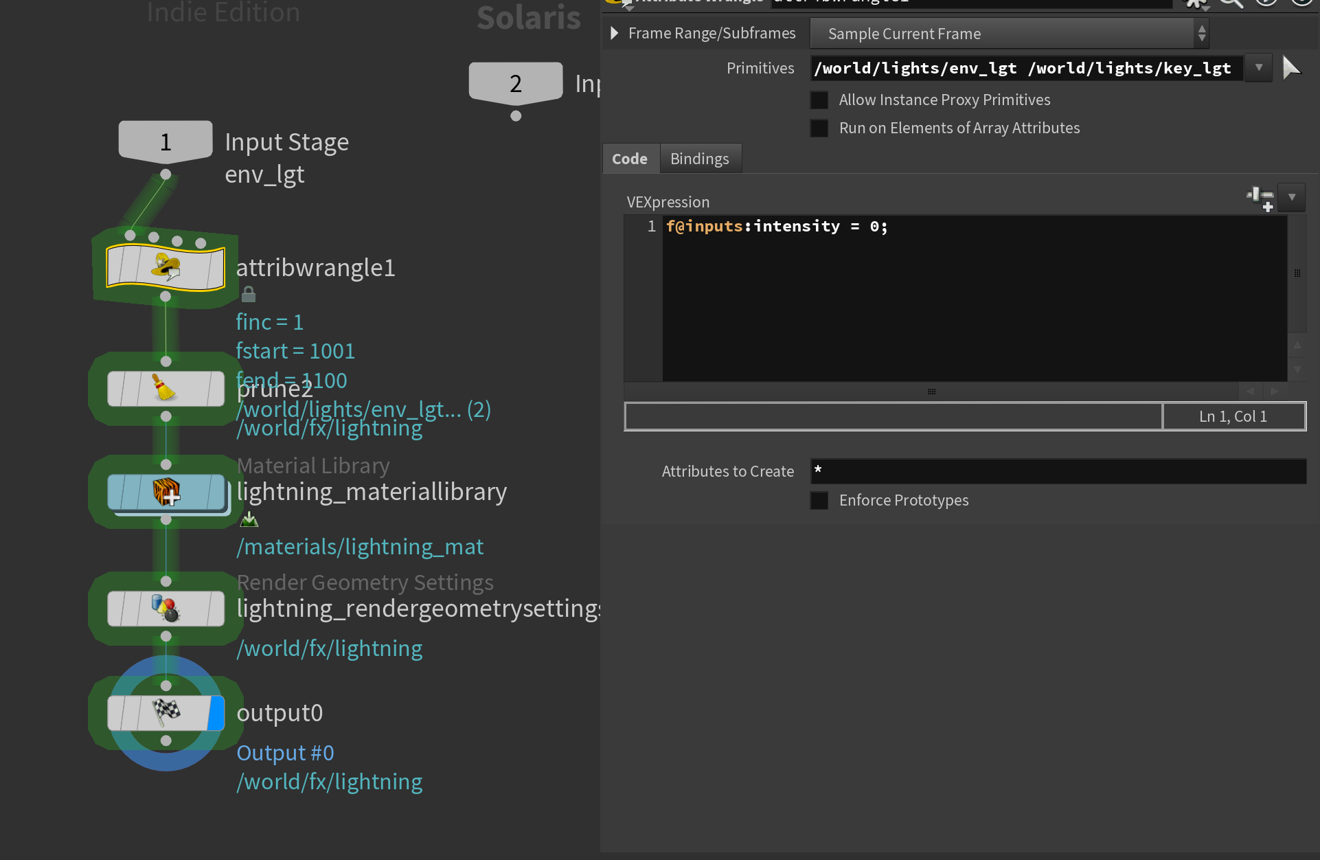
First, in the Wrangle node, I set the intensity of the lights to 0 using a VEX expression. I originally wanted to just prune the lights, but I couldn't get rid of Karma's headlights (default lights when no lights are present) - for some reason disabling the creation of that did nothing. Therefore I resorted to this.
Following that I un-pruned our lightning primitive. Remember how we deactivated it earlier in the network? Now we're re-enabling it by setting the method to Deactivate and setting the Prune parameter to 0. Now our lightning is present in our scene again.
Then, inside a Material Library, I create a Karma Material Builder and turn off everything inside the generated Mtlx Standard Surface except for emission, which I set to 10,000. This is necessary to create a geometry light with Karma.
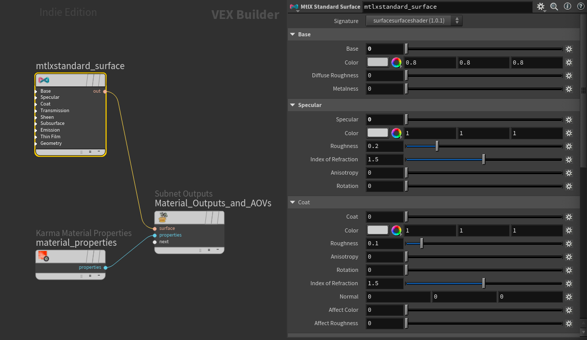
I then apply the shader to the lightning inside the Material Library like so:
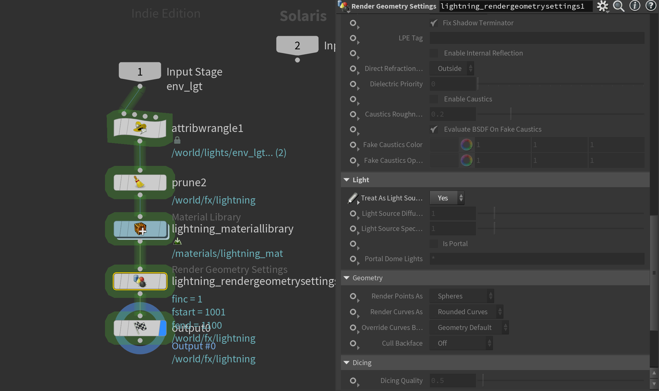
Finally, I set the lightning geometry to be a proper geometry light by adding a Render Geometry Settings, targeting the lightning primitive, and setting Treat As Light Source to Yes.
Please note that you'll need to apply an emission shader like the above first for this to work properly.
For the render settings, I'm using almost the same as my beauty render layer, except I'm boosting the Volume Limit to 32 and Path Traced Samples to 512 as I found it gave me the best results.
After this, I append a USD Render ROP as I did with the beauty and render only the frames where my lightning is active.
Compositing
with Nuke
Now we're in the home stretch! If you've followed the tutorial until this point I commend you, this is the longest article I've written so far. Thank you for sticking with it.
I got some requests in my previous tutorials to cover compositing as well, so I'm diving into a bit more detail here than last time. This shot has received more comp treatment than I usually do in my personal work, so I hope you pick up some useful tricks.
Beauty treatment
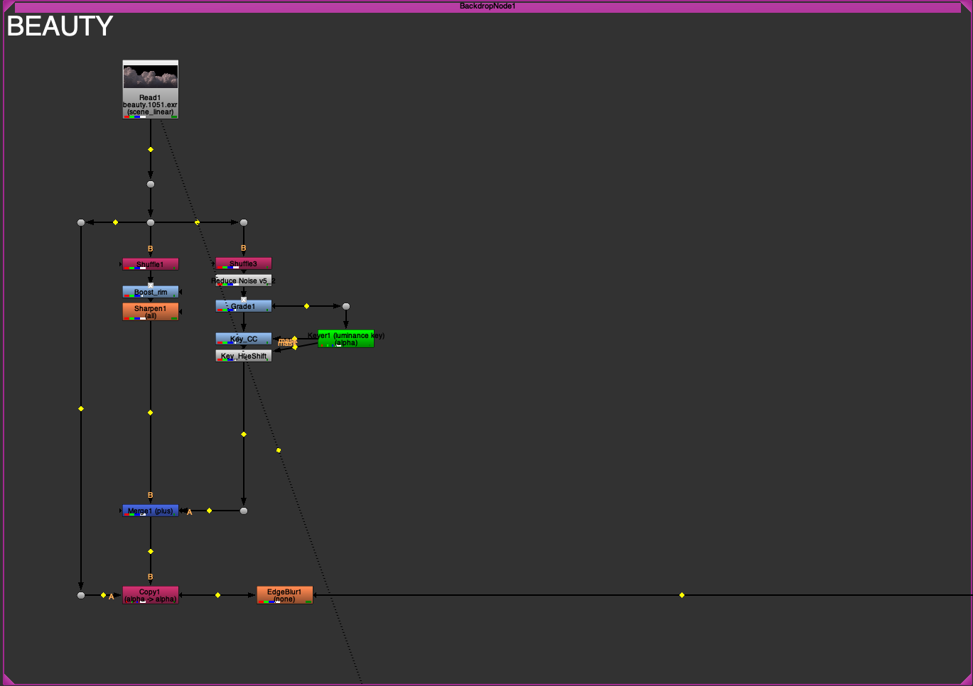
For the beauty renderlayer, I made some fairly heavy grades to push it that extra 10 - 20 %. You can see the final result below. If you need to get an overview of the node network you can refer to the screenshot above.
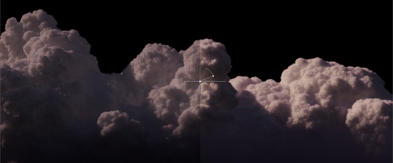
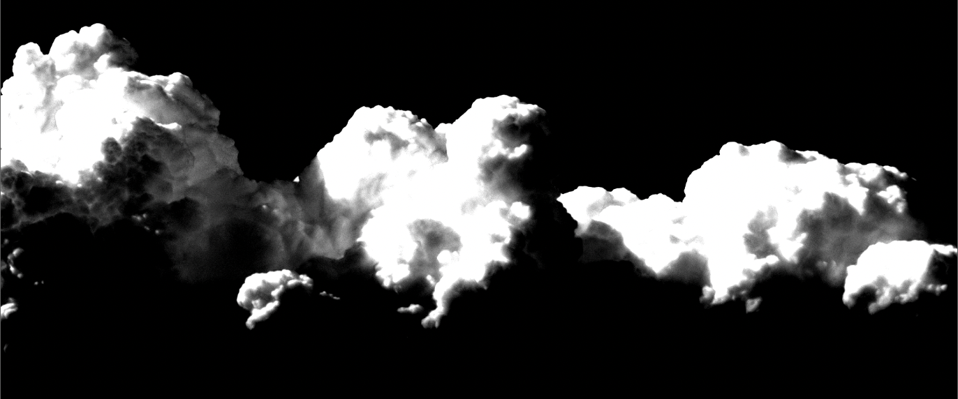
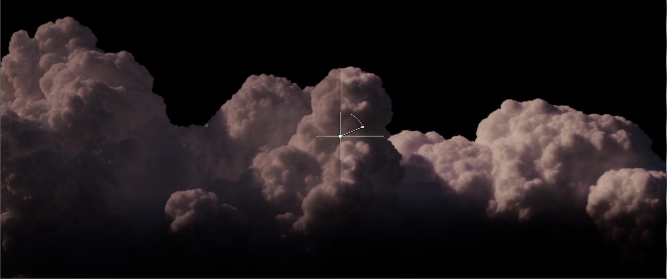
The first thing I did was split my beauty into Direct and Indirect lighting using the AOVs we created using Karma. This will be important especially since I wanted to denoise the indirect lighting AOV.
As you can see below the Indirect Lighting AOV defines most of the look, but the Direct Lighting is useful as it can help provide a bit more shaping to our clouds (so the model doesn't get lost in scattering).
For grading my best tip is always to pull in some great reference from movies or photography and use Nuke's viewer info/eye dropper tool to sample what values they used.
Direct Lighting
For the Direct Lighting grade, I simply boosted the contrast by lowering the white point and increasing the black point slightly. Then, using a sharpen node set to a very low amount I increased the details a little bit, just to make the clouds a bit less soft.
Indirect Lighting
The Indirect lighting has a bit more complexity in its treatment as I also decided to denoise it.
The denoising was done using the Neat Video Reduce Noise plugin. I'm not affiliated with this company, but their plugin is often used in VFX studios to denoise footage/plates. It has the side-effect of also being quite efficient at denoising renders. So that's what I'm using it for here.
Then I did a subtle grade pushing some of the orange out a bit more through a colored gain in a grade node, followed by a color correct using a lumakey as a mask to boost the brightest values significantly and performing a hueshift to closer match my reference.
Finally, I added this pass together with my Direct Lighting using a plus operation in a merge, copied over my alpha from the original beauty, and performed a subtle edge blur to soften some of the edges. This gave me the final result below. Refer to the node network screenshot earlier to see the exact connections.
Background
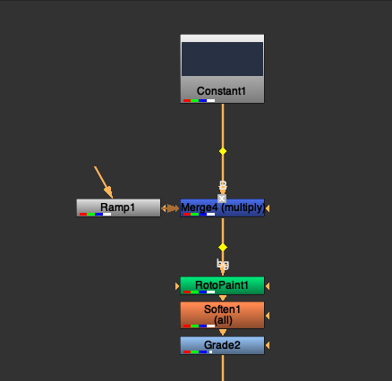
I created a very simple background in this shot directly in Nuke as I felt it was all I needed in this particular instance. I created it using a constant set to a color I sampled from my reference and multiplied that with a ramp darkening the top of the frame.
Following that I painted a couple of 1-pixel stars using a RotoPaint node and added a soften to blur them a tiny bit. Finally, I added a grade to darken everything a bit more - just to make it fit better with the beauty.

I used this in a regular A over B merge operation with the beauty. Remember to make sure that the background has an alpha.
Lightning
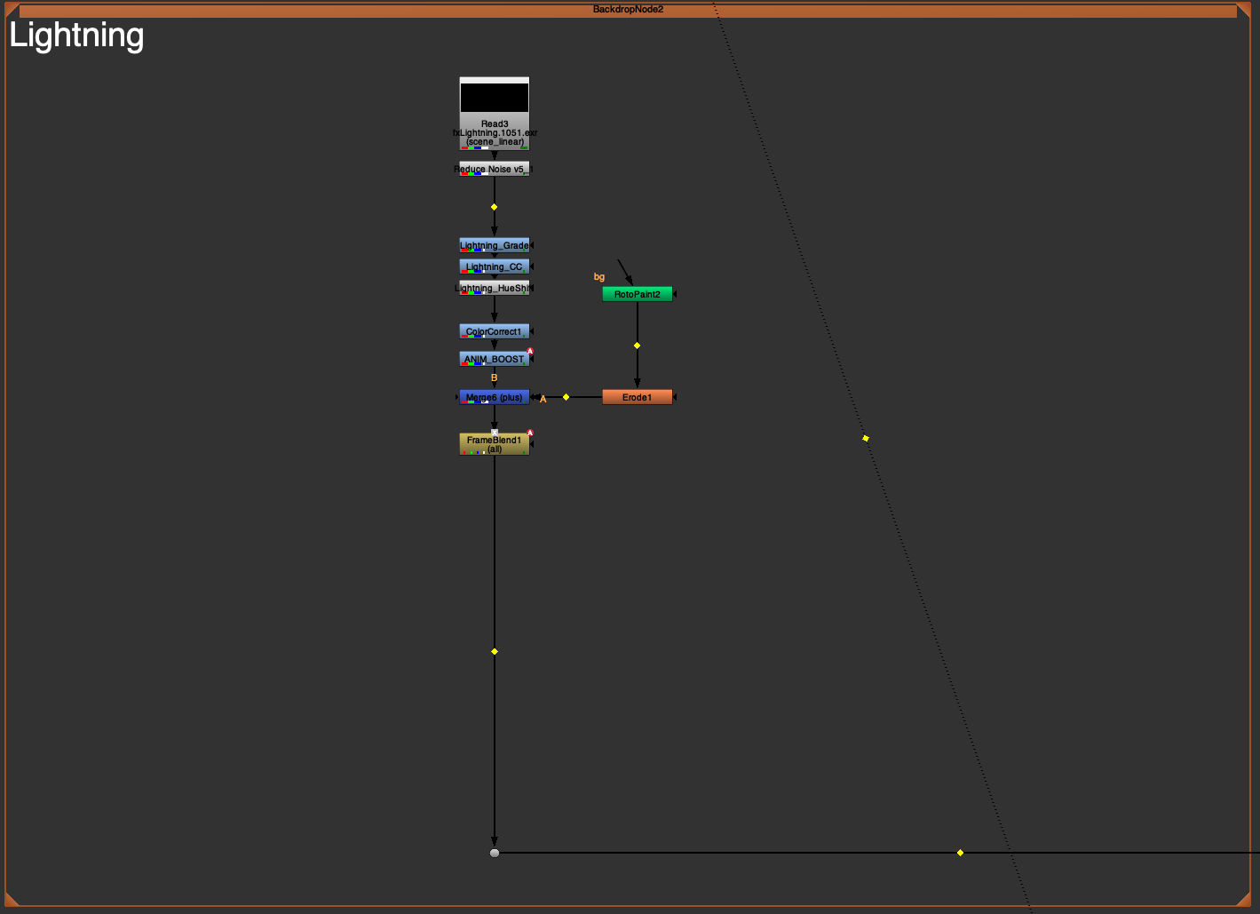
The lightning layer ended up being added (using a plus operation on a merge node) on top of the beauty - this allowed me to grade the lightning individually to tweak the look.
First I did another denoise on the lightning layer using a Reduce Noise node like earlier. I then graded the lightning strikes globally using a series of color corrects, grades, and hue shifts.

One thing to note here is that I animated the gain of one of the grade nodes. This was to grade some of the lightning strikes individually as some of them were a bit too faint.
I also painted a single lightning strike on one frame using a RotoPaint node followed by an erode (to shrink its thickness a bit). This was to fix a lightning geometry that wasn't bright enough. Normally I would have created a utility layer with an alpha for this lightning strike, but since it was just one frame I settled with some manual labor. This was added on top of the lightning render layer.
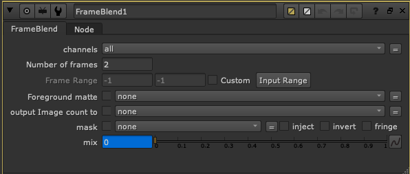
Before adding this to our full compositing stream I added a frameblend. This was to achieve an extra "ghosting" frame for each lightning strike. I set the Number of Frames to 2 and animated the mix to only be 1 on the frame directly after the lightning strike hits in the render.
Finally, I merged this into my main stream using a merge operation set to plus.
Final details
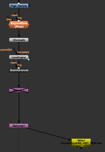
To finish the shot I added some final details. First I did a grade node lowering the gamma a bit (to push contrast slightly).
Then I used several Nuke Gizmos including Chromatik, Exponential Glow, Lens Engine, and Grain Advanced to add chromatic aberration, a bit of glow, a very subtle vignette, and some film grain. All these nodes can be found in the excellent free Nuke Survival Toolkit.
I added a reformat at the end to make sure I didn't have any stray bounding boxes.
Final composited shot.
Conclusion
And that wraps up this tutorial! Thanks again for reading, this was quite a long one to write so I appreciate you checking it out. If you have any questions or comments feel free to reach out in the comment section below.
If you're interested in more content like this consider subscribing to my newsletter below. You'll get every post I release directly to your inbox.